How to model discrete growth

library(cmdstanr)
library(ggplot2)
library(tidyverse)
library(tidybayes)
library(targets)

tar_load(one_time)
plot(one_time, type = "l")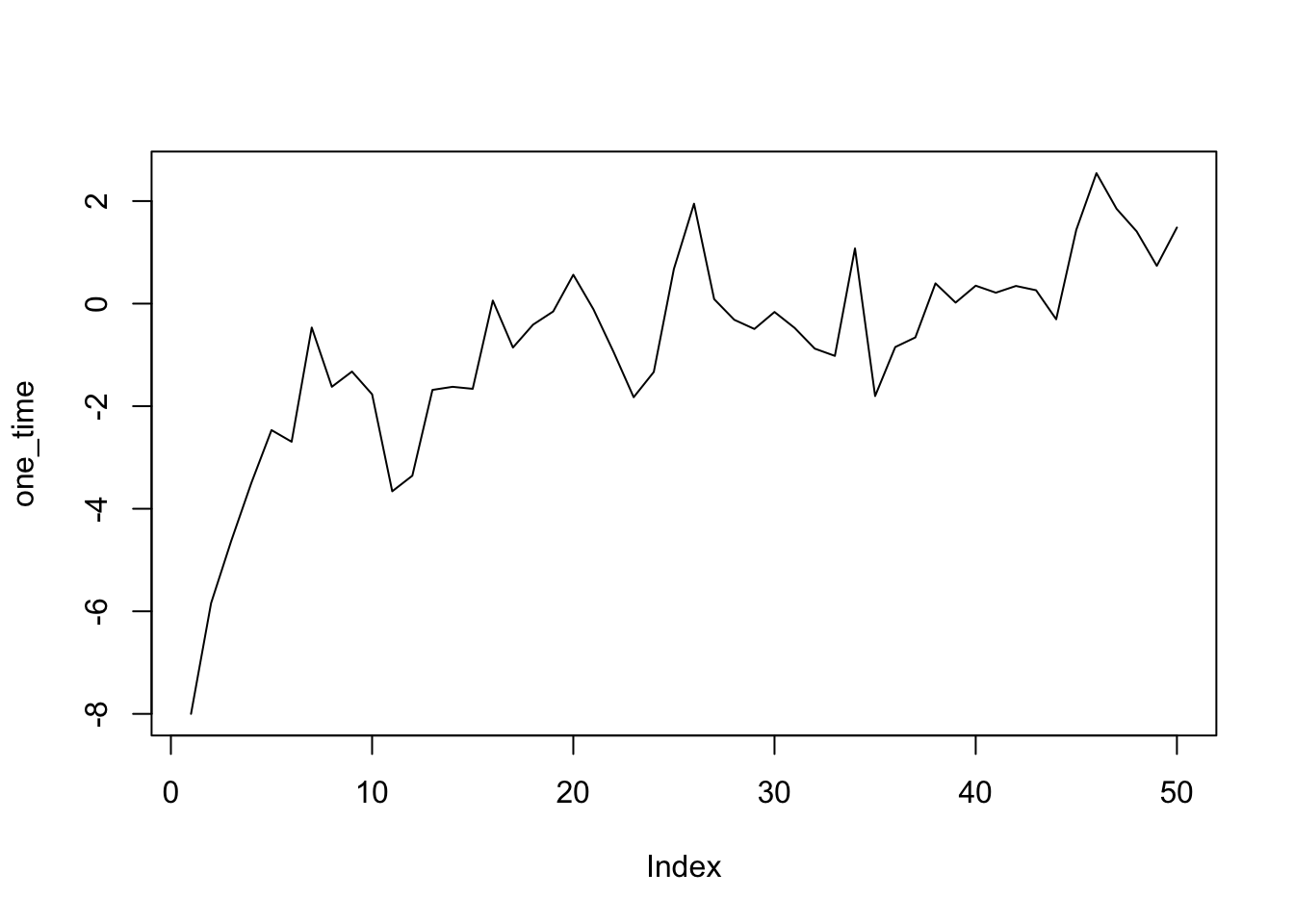

Controversy!

# load the model in stan
transition <- cmdstan_model(here::here("posts/2023-11-24-how-to-model-growth/ar1.stan"))

transition

data{
  int n;
  vector[n] time;
  vector[n] x;
}
// transformed data {
//   vector[n] x = log(pop);
// }
parameters {
  real<lower=0> a;
  real<lower=0,upper=1> b;
  real<lower=0> sigma;
}
transformed parameters {
  real mu_max = a / (1 - b);
  real sigma_max = sigma /sqrt(1 - b^2);
}
model {
  a ~ normal(2, .5);
  b ~ beta(5,2);
  sigma ~ exponential(5);
  x ~ normal(
    mu_max .* (1 - pow(b, time)),
    sigma_max .* sqrt(1 - pow(b^2, time))
    );
}
generated quantities {
  vector[15] x_pred;
  x_pred[1] = 0;
  for (j in 1:14) {
    x_pred[j+1] = normal_rng(
      mu_max * (1 - pow(b, j)),
      sigma_max * sqrt(1 - pow(b^2, j))
      );
  }
}

Here is another approach, using a lagged population growth model

# load the model in stan
lagged_growth <- cmdstan_model(here::here("posts/2023-11-24-how-to-model-growth/multiple_spp_ar1.stan"))

lagged_growth

data {
  int n;
  int nclone;
  vector[n] x;
  array[n] int<lower=1, upper=nclone> clone_id;
  // for predictions
  int<lower=0, upper=1> fit;
  int nyear;
}
transformed data {
  array[n - nclone] int time;
  array[n - nclone] int time_m1;
  for (i in 2:n) {
    if (clone_id[i] == clone_id[i-1]) {
      time[i - clone_id[i]] = i;
      time_m1[i - clone_id[i]] = i - 1;
    }
  }
}
parameters {
  real<lower=0> a;
  real<lower=0,upper=1> b;
  real<lower=0> sigma;
}
model {

  a ~ normal(2, .5);
  b ~ beta(5,2);
  sigma ~ exponential(5);

  if (fit == 1) {

    x[time] ~ normal(
      a + b * x[time_m1],
      sigma);
  }
}
generated quantities {
  vector[nyear] x_pred;

  x_pred[1] = 0;

  for (j in 2:nyear){
    x_pred[j] =  a + b * x_pred[j-1] + normal_rng(0, sigma);
  }
}

Simulations

Here are simulations from a one-species AR-1 model that imitate Ives et al. figure 1.

simulate_pop_growth <- function(
    a = 0, 
    b, 
    sigma = 1, 
    tmax = 50, 
    x0 = -8) {
  
  xvec <- numeric(tmax)
  
  xvec[1] <- x0
  
  ## process error
  eta <- rnorm(tmax, mean = 0, sd = sigma)
  
  for(time in 2:tmax){
    xvec[time] <- a + b*xvec[time-1] + eta[time]
  }
  
  return(xvec)
}

I’m going to simulate a modest number of time series, and choose parameters to make the time series slightly resemble the aphid experiment.

a_fig = 1
b_fig = .8
sigma_fig = .7

ts_data <- map_dfr(1:12, 
        ~ tibble(
          pop = simulate_pop_growth(
            a = a_fig, 
            b = b_fig,
            tmax = 16, 
            sigma = sigma_fig, 
            x0 = 0
            ),
          time = 0:(length(pop)-1)
        ),
        .id = "sim"
)

ts_data |> 
  ggplot(aes(x =time, y = pop, group = sim)) + 
  geom_line()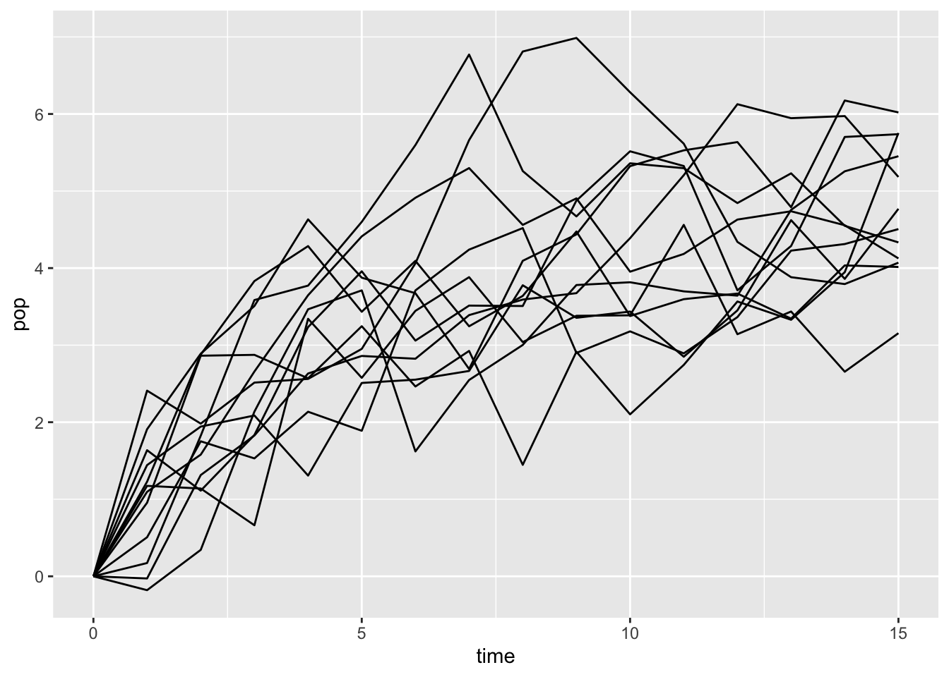

knitr::kable(head(ts_data))

sim	pop	time
1	0.0000000	0
1	0.9548568	1
1	2.8629644	2
1	2.8740721	3
1	2.5695696	4
1	3.2455612	5

Transition distribution

ts_data_nozero <- filter(ts_data, time != 0)


transition_sample <- transition$sample(
  data = list(n = nrow(ts_data_nozero),
              x = ts_data_nozero$pop,
              time = ts_data_nozero$time),
  parallel_chains = 4, refresh = 0)

Running MCMC with 4 parallel chains...

Chain 1 finished in 1.7 seconds.
Chain 3 finished in 1.7 seconds.
Chain 2 finished in 1.8 seconds.
Chain 4 finished in 1.7 seconds.

All 4 chains finished successfully.
Mean chain execution time: 1.7 seconds.
Total execution time: 2.0 seconds.

transition_sample |> 
  spread_rvars(x_pred[time]) |> 
  ggplot(aes(x = time-1, ydist = x_pred)) + 
  stat_lineribbon() + 
  scale_fill_brewer(palette = "Greens", direction = -1) + 
  theme_bw() + 
  geom_line(aes(x = time, y = pop, group = sim),
            inherit.aes = FALSE, data = ts_data) + 
  labs(x = "Time", y = "log population size")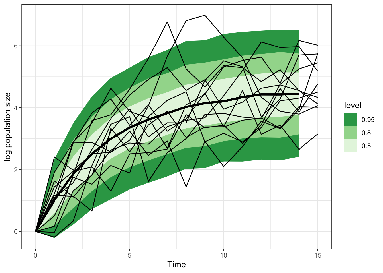

transition_sample |>
  gather_rvars(a, b, sigma) |> 
  ggplot(aes(y = .variable, dist = .value)) + 
  stat_halfeye() + 
  geom_point(
    aes(y = .variable,  x = .value),
    inherit.aes = FALSE,
    data = tribble(
      ~ .variable, ~.value,
      "a", a_fig, 
      "b", b_fig,
      "sigma", sigma_fig), col = "red", size = 2)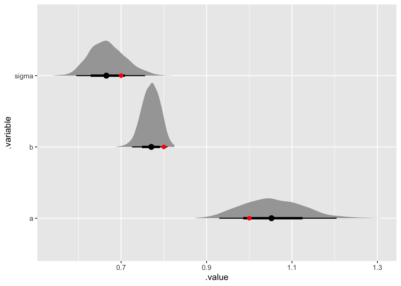 

Lagged model

This time there is no need to drop 0s

ts_data <- ts_data |> 
  mutate(sim = readr::parse_number(sim))

lagged_growth_sample <- lagged_growth$sample(
  data = list(n = nrow(ts_data),
              nclone = max(ts_data$sim),
              x = ts_data$pop,
              time = ts_data$time,
              clone_id = ts_data$sim,
              fit = 1,
              nyear = 15),
  parallel_chains = 4, refresh = 0)

Running MCMC with 4 parallel chains...

Chain 1 finished in 0.3 seconds.
Chain 2 finished in 0.3 seconds.
Chain 3 finished in 0.3 seconds.
Chain 4 finished in 0.3 seconds.

All 4 chains finished successfully.
Mean chain execution time: 0.3 seconds.
Total execution time: 0.5 seconds.

predictions

lagged_growth_sample |> 
  spread_rvars(x_pred[time]) |> 
  ggplot(aes(x = time-1, ydist = x_pred)) + 
  stat_lineribbon() + 
  scale_fill_brewer(palette = "Greens", direction = -1) + 
  theme_bw() + 
  geom_line(aes(x = time, y = pop, group = sim),
            inherit.aes = FALSE, data = ts_data) + 
  labs(x = "Time", y = "log population size")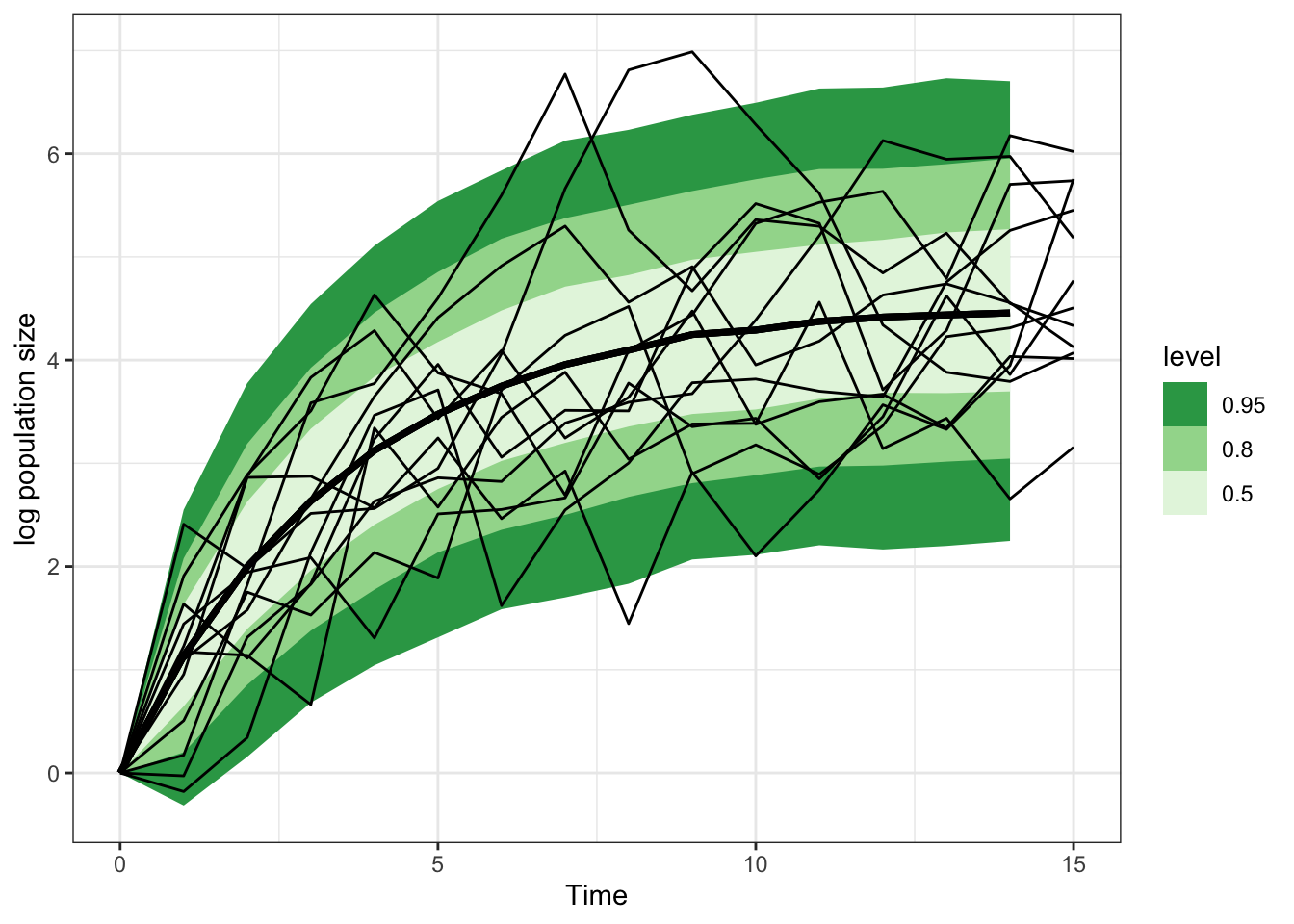

parameters

lagged_growth_sample |>
  gather_rvars(a, b, sigma) |> 
  ggplot(aes(y = .variable, dist = .value)) + 
  stat_halfeye() + 
  geom_point(
    aes(y = .variable,  x = .value),
    inherit.aes = FALSE,
    data = tribble(
      ~ .variable, ~.value,
      "a", a_fig, 
      "b", b_fig,
      "sigma", sigma_fig), col = "red", size = 2)