Discrete-time population growth in Stan

library(cmdstanr)
library(ggplot2)
library(tidyverse)
library(tidybayes)

Background

How do species populations change over time?

How much of that change is caused by interactions with their community?

20 years ago a very influential paper was written by Ives, Dennis, Cottingham and Carpenter (Ives et al. 2003). Ives et al. present a method called a first-order Multivariate AutoRegressive model, also known as MAR(1). The core idea is that species are growing in a density-dependent way, but at a rate that is influenced by the per-capita effects of every other interacting population. A transition matrix captures the effects of each species on every other, and lets us predict how the vector species abundances changes over time.

Ives et al. advance this argument by beginning with univariate (single-species) approach, and that is what this post is about. Perhaps a future post will cover all the models.

\[ \begin{align} n_t &= n_{t - 1}e^{a + (b - 1)ln(n_{t-1})} \\ ln(n_t) = x_t &= a + bx_{t - 1} \end{align} \] We can predict the curve at any time \(t\) with this expression, from finite series:

\[ x_t = x_\infty + b^t(x_0 - x_\infty) \]

curve(200 + (.9)^x * (4 - 200), xlim = c(0, 100))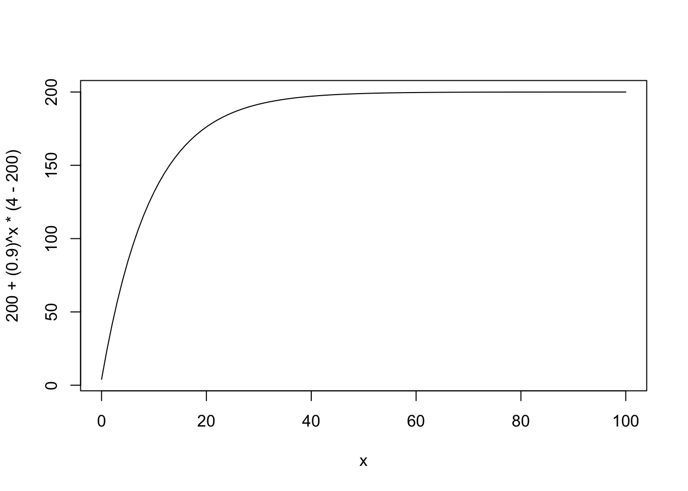

Curve of a Gompertz growth model.

However there might be variation every time step because growth rate differences are caused by lots of unmeasured things.

\[ \begin{align} X_t &= a + bX_{t-1} + \epsilon_t \\ \epsilon &\sim \text{Normal}(0, \sigma) \end{align} \]

This leads to a mean and variance at time \(t = \infty\)

\[ \begin{align} \mu_\infty &= \frac{a}{1 - b} \\ v_\infty &= \frac{\sigma^2}{1 - b^2} \end{align} \]

and the mean and variance at time \(t\)

\[ \begin{align} \mu_t &= \mu_\infty + b^t(x_0 - \mu_\infty) \\ v_t &= \sigma^2\frac{1 - (b^2)^t}{1 - b^2} = v_\infty(1 - b^{2t}) \end{align} \] Everything here is on the log scale. The result is something that we can work with in a model for the likelihood – the mean and variance of a normal distribution.

Simulations

Here are simulations from a one-species AR-1 model that imitate Ives et al. figure 1.

simulate_pop_growth <- function(
    a = 0, 
    b, 
    sigma = 1, 
    tmax = 50, 
    x0 = -8) {
  
  xvec <- numeric(tmax)
  
  xvec[1] <- x0
  
  ## process error
  eta <- rnorm(tmax, mean = 0, sd = sigma)
  
  for(time in 2:tmax){
    xvec[time] <- a + b*xvec[time-1] + eta[time]
  }
  
  return(xvec)
}

map_dfr(1:10, ~ tibble(pop = simulate_pop_growth(b = 0.6, tmax = 50),
                       time = 1:length(pop)), .id = "sim") |> 
  ggplot(aes(x = time, y = pop, group = sim)) + 
  geom_line() + 
  geom_hline(yintercept = 0) + 
  theme_bw()
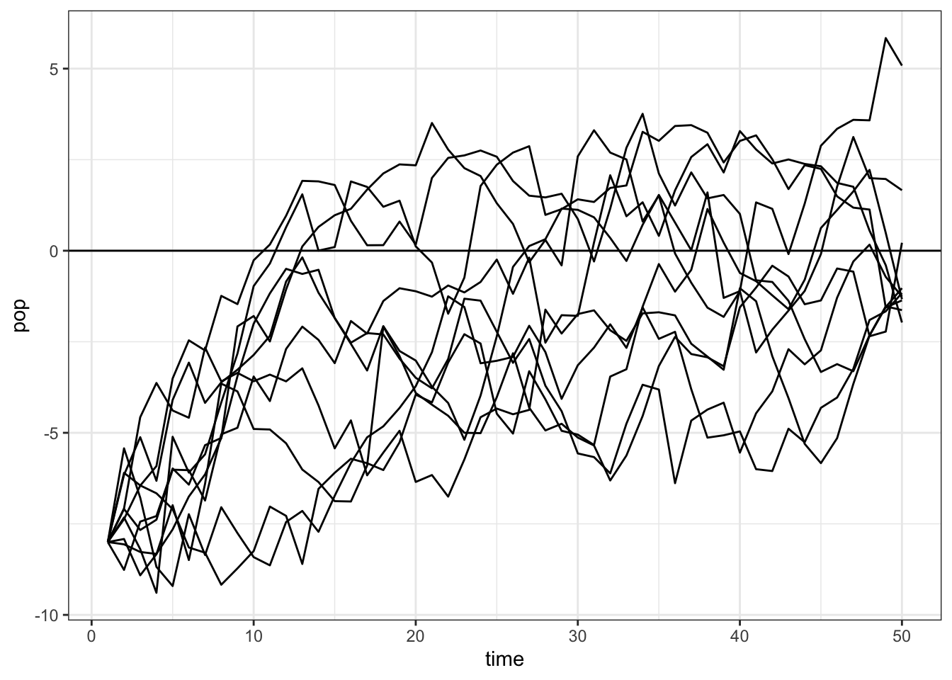
map_dfr(1:10, ~ tibble(pop = simulate_pop_growth(b = 0.95, tmax = 50),
                       time = 1:length(pop)), .id = "sim") |> 
  ggplot(aes(x = time, y = pop, group = sim)) + 
  geom_line() + 
  geom_hline(yintercept = 0)+ 
  theme_bw()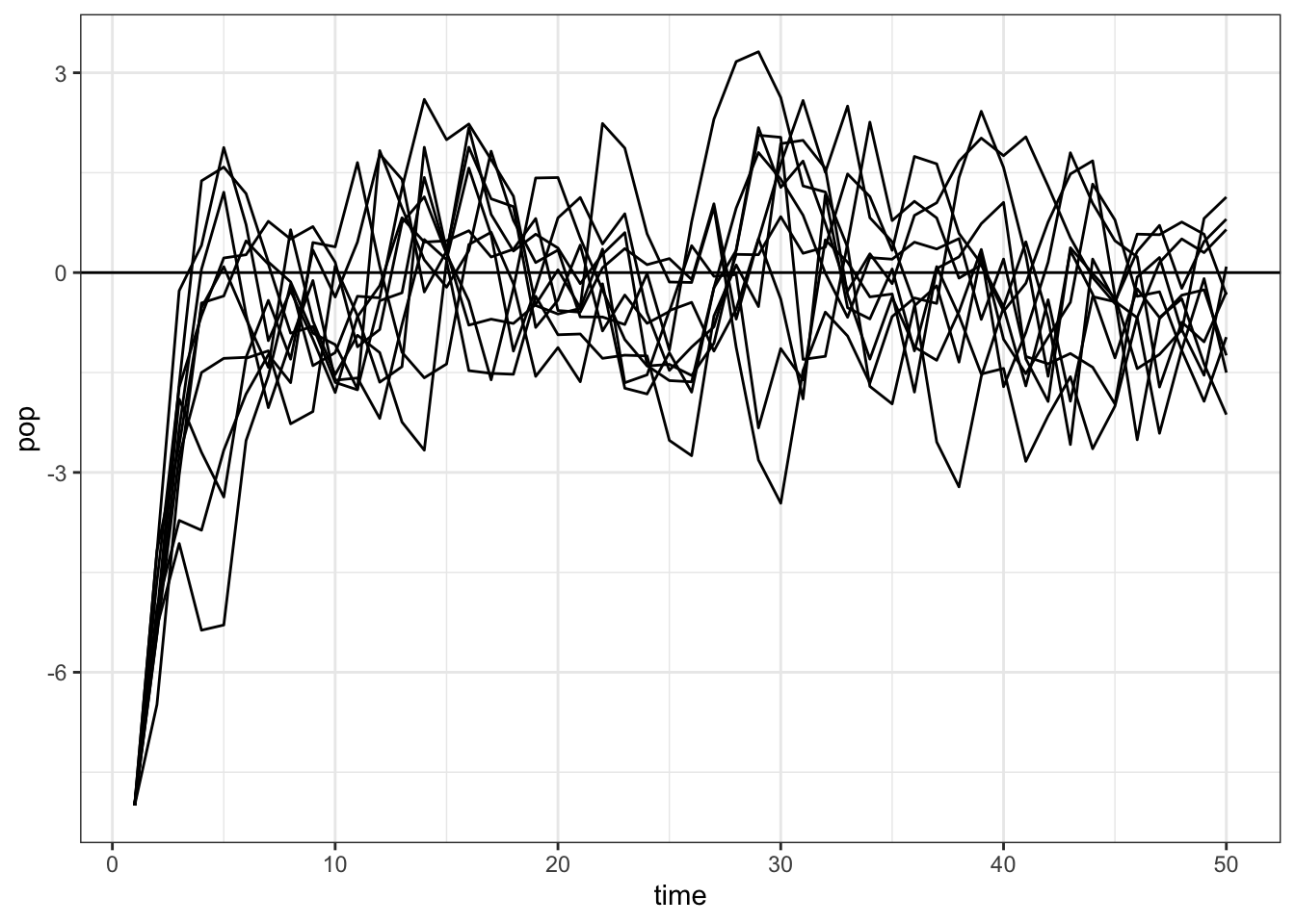

Growth with a = 0, b = .6, sigma = 1

Growth with a = 0, b = .95, sigma = 1

It’s fun to take a look at this curve after exponentiating it, so as to see the real population sizes.

map_dfr(1:10, 
        ~ tibble(pop = simulate_pop_growth(
          a = 3, b = 0.4, tmax = 10, sigma = 0.03),
          time = 1:length(pop)), .id = "sim") |> 
  ggplot(aes(x = time, y = exp(pop), group = sim)) + 
  geom_line() + 
  geom_hline(yintercept = 0, lty = 2)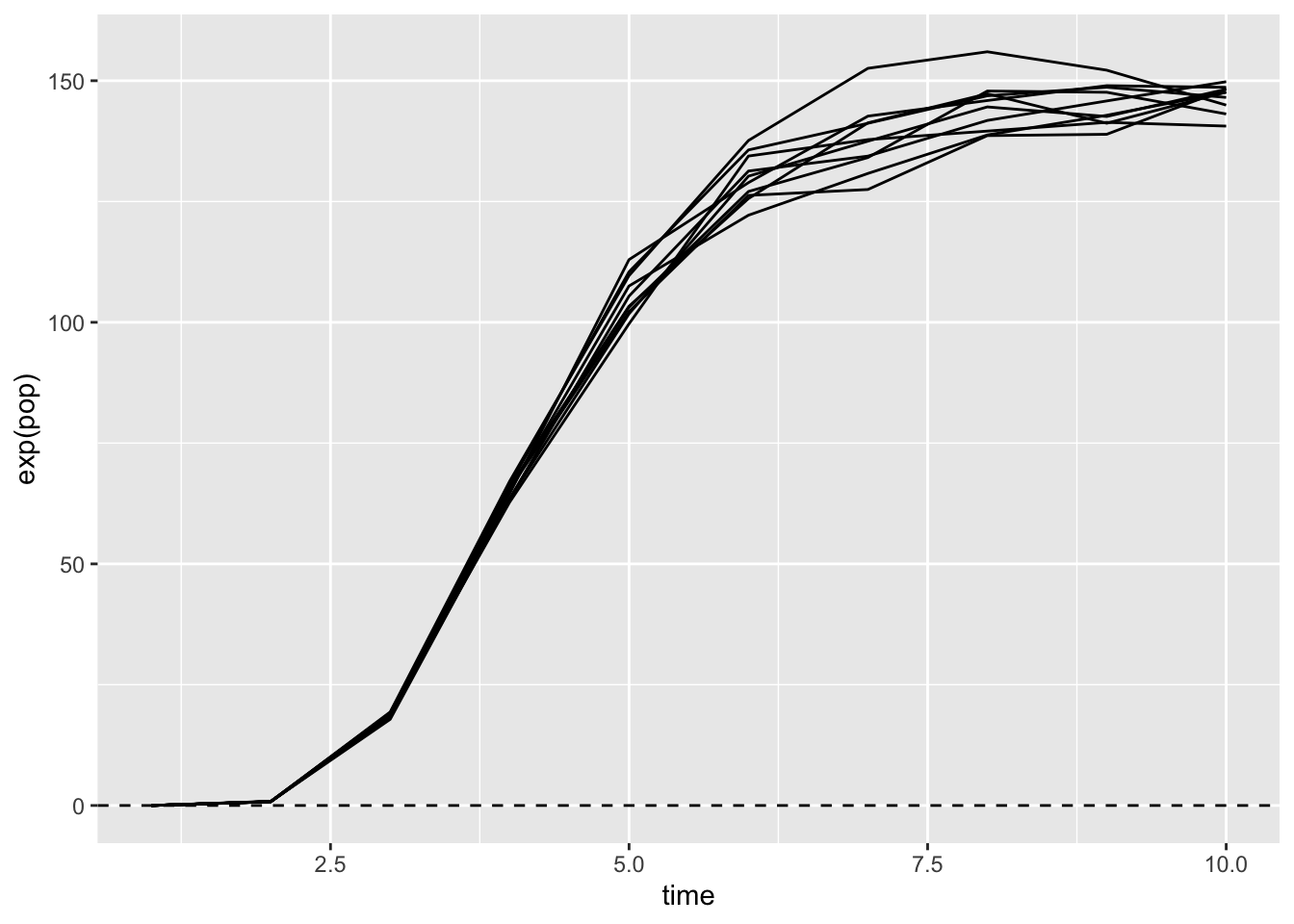

Functions for the mean and variance

We can also get a plot of the changing mean and variance over time. Just from playing with these, we can see what the simulations earlier showed: that variance depends on both the process error \(\sigma\) and on the parameter that controls the amount of density dependence, \(b\).

calc_mean <- function(a, b, time, n_start){
  mu_max <- a / (1 - b)
  
  mu_max + b^time * (n_start - mu_max)
}

calc_var <- function(b, time, sigma){
  bsq <- b^2
  
  var_max = sigma^2/(1 - bsq)
  
  var_max * (1 - bsq^time)
}

curve(calc_mean(0, .8, n_start = -8, time = x), xlim = c(0, 50))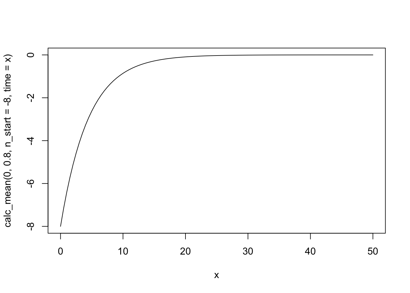

curve(calc_var(.9, time = x, sigma = 1),
      xlim = c(0,50), ylim = c(0, 10))

curve(calc_var(.8, time = x, sigma = 1), add = TRUE)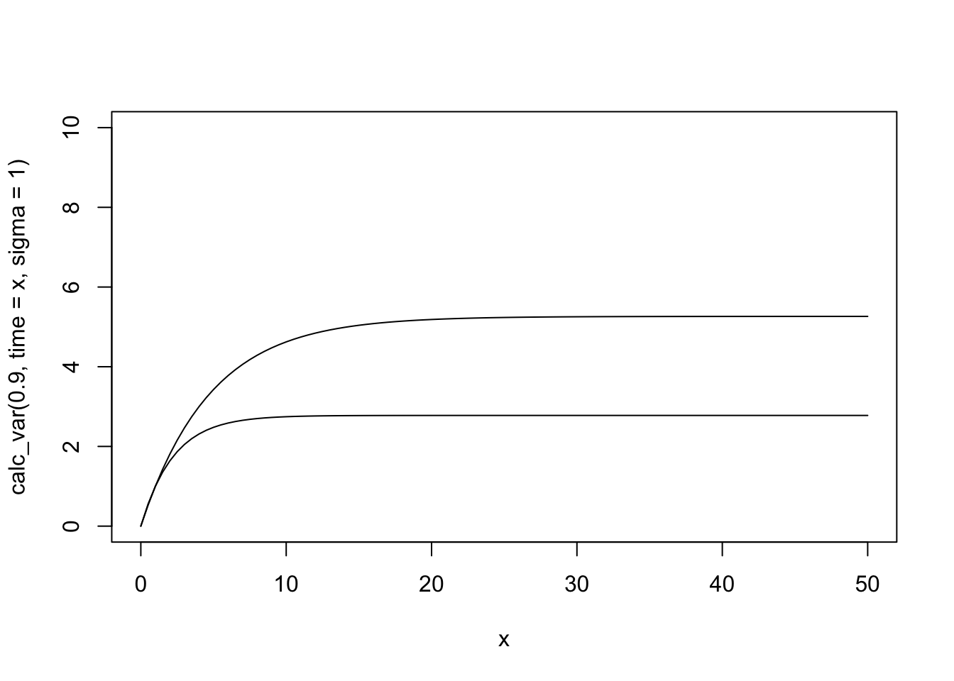

Do these numbers reflect the distribution we see in the simulations?

set.seed(5002)
some_sims <- map_dfr(1:300, ~ tibble(pop = simulate_pop_growth(b = 0.9, tmax = 30),
                       time = 0:(length(pop)-1)), .id = "sim")

sim_meanvar <- some_sims |> 
  group_by(time) |> 
  summarize(sim_mean = mean(pop),
            sim_var = var(pop))

some_sims |> 
  filter(time == 22) |> 
  pluck("pop") |> 
  hist(probability = TRUE, breaks = 30, xlab = "population size (log)", main = "Simulated and predicted population size distribution")

curve(dnorm(x, 
            mean = calc_mean(a = 0, b = .9, time = 22, n_start = -8),
            sd = sqrt(calc_var(b = .9, time = 22, sigma = 1))), 
      add = TRUE)
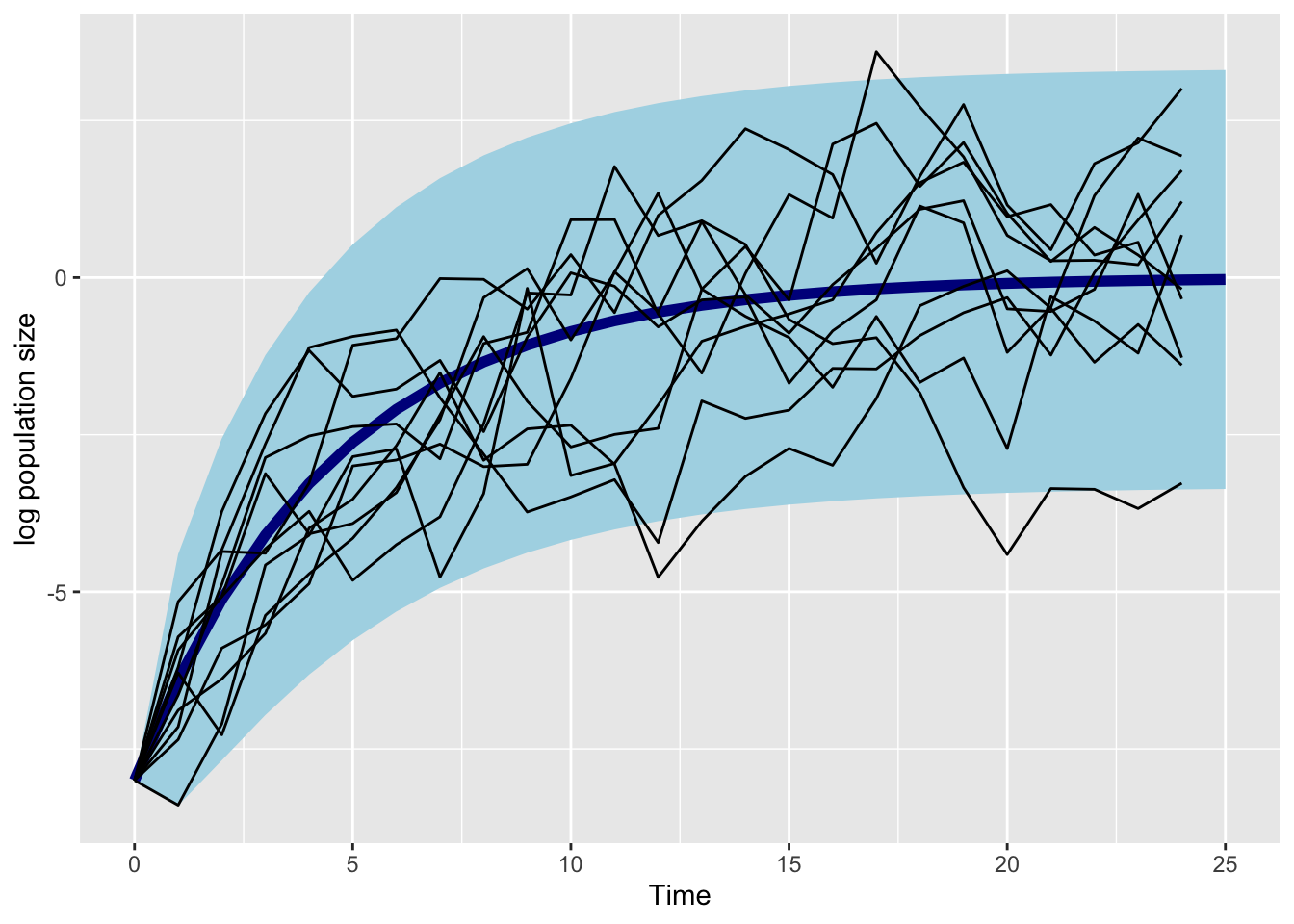
a_fig <- 0
b_fig <- 0.8
nstart_fig <- -8
sigma_fig <- 1

tibble(
  time = 0:25,
  mean = calc_mean(
    a = a_fig, b = b_fig, time = time,
    n_start = nstart_fig),
  sd = sqrt(calc_var(
    b = b_fig, time = time, sigma = sigma_fig))) |> 
  ggplot(aes(x = time,
             ymin = mean - sd*2,
             ymax = mean + sd*2, 
             y = mean)) + 
  geom_ribbon(fill = "lightblue")+
  geom_line(col = "darkblue", lwd = 2) + 
  geom_line(
    aes(x = time,
        y = pop, 
        group = sim),
    inherit.aes = FALSE,
    data = map_dfr(1:10, 
                   ~ tibble(
                     pop = simulate_pop_growth(
                       a = a_fig, 
                       b = b_fig,
                       tmax = 25, 
                       sigma = sigma_fig),
                     time = 0:(length(pop)-1)
                     ),
                   .id = "sim"
                   )
  ) + 
  NULL + 
  labs(x = "Time", y = "log population size")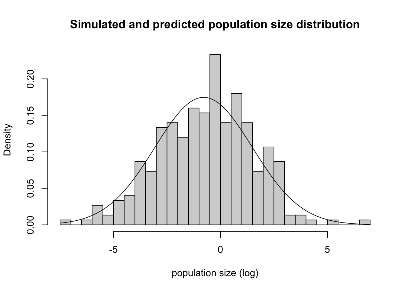

Simulations match the theoretical predictions very closely. Math works!

Simulations match the theoretical predictions very closely. Math works!

Aphids

Below I explore this model and try to fit some examples in Stan. I’m building this example to match work being done at UdeS by students of Matt Barbour. In these experiments, a single aphid is placed on a radish plant. Aphids are clonal, and give birth to live (!) young.

Each colony, incredibly, starts with a single aphid. This simplifies the expressions for the average and the variance because the starting population size is \(ln(1) = 0\)

\[ \begin{align} \mu_t &= a\frac{1 - b^t}{1 - b} &= \mu_\infty(1 - b^t) \\ v_t &= \sigma^2\frac{1 - (b^2)^t}{1 - b^2} &= v_\infty(1 - b^{2t}) \end{align} \]

The entire experiment fits on a single tray in a growth chamber, and Katerie replicated the experiment 6 times.

Math: a model for one clone

When we are making replicates observations of a single clone, we only need to know four quantites to predict both the average and the variation around that average: \(a\), \(b\), \(\sigma\) and the time that passed since the start, \(t\)

Here is the full Bayesian model with priors. I used prior simulations to come up with these numbers (that’s the next section below!)

\[ \begin{align} x_{i} &\sim \text{Normal}(\mu_t, \sqrt{v_t})\\ \mu_t &= \mu_\infty(1 - b^t) \\ v_t &= v_\infty(1 - b^{2t}) \\ \mu_\infty &= \frac{a}{1 - b} \\ v_\infty &= \frac{\sigma^2}{1 - b^2} \\ a &\sim \text{Normal}(2, .5) \\ b &\sim \text{Beta}(5, 2) \\ \sigma &\sim \text{Exponential}(1) \\ \end{align} \]

Make fake data

Simulating from the data-generating model

sim_one_gompertz <- function(K = 1000, 
         a = 1, 
         b = 0.86,
         s = .3,
         ntime = 15){
  
  N = c(0, 
        rnorm(ntime - 1, 
              mean = a * (1 - b^(1:(ntime-1))) / (1 - b),
              sd = s * (1 - (b^2)^(1:(ntime-1))) / (1 - b^2)
        )
  )
        
        
  return(tibble(N = N, time = 0:(ntime-1)))
}

map_df(1:6, ~ list(sim_one_gompertz()), .id = "sim_id") |> 
  ggplot(aes(x = time, y = N, group = sim_id)) + 
  geom_line()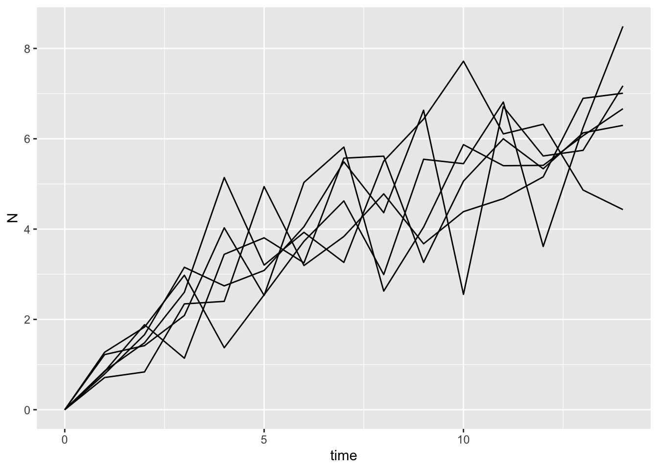

# load the model in stan
ar_1 <- cmdstan_model(here::here("posts/2023-11-15-ives03-ts/ar1.stan"))

ar_1

data{
  int n;
  vector[n] time;
  vector[n] x;
}
// transformed data {
//   vector[n] x = log(pop);
// }
parameters {
  real<lower=0> a;
  real<lower=0,upper=1> b;
  real<lower=0> sigma;
}
transformed parameters {
  real mu_max = a / (1 - b);
  real sigma_max = sigma /sqrt(1 - b^2);
}
model {
  a ~ normal(2, .5);
  b ~ beta(5,2);
  sigma ~ exponential(5);
  x ~ normal(
    mu_max .* (1 - pow(b, time)),
    sigma_max .* sqrt(1 - pow(b^2, time))
    );
}
generated quantities {
  vector[15] x_pred;
  x_pred[1] = 0;
  for (j in 1:14) {
    x_pred[j+1] = normal_rng(
      mu_max * (1 - pow(b, j)),
      sigma_max * sqrt(1 - pow(b^2, j))
      );
  }
}

gomp_one_pop_df <- map_df(1:6, ~ list(
  sim_one_gompertz()), .id = "sim_id")
  
  
gomp_nozero <- gomp_one_pop_df  |> 
    filter(time != 0)

gomp_ar_1_sample <- ar_1$sample(data = list(n = nrow(gomp_nozero),
                        x = gomp_nozero$N,
                        time = gomp_nozero$time),
                        parallel_chains = 4, refresh = 0)

Running MCMC with 4 parallel chains...

Chain 2 finished in 0.9 seconds.
Chain 1 finished in 1.0 seconds.
Chain 3 finished in 0.9 seconds.
Chain 4 finished in 0.9 seconds.

All 4 chains finished successfully.
Mean chain execution time: 0.9 seconds.
Total execution time: 1.2 seconds.

gomp_ar_1_sample |> 
  spread_rvars(x_pred[time]) |> 
  ggplot(aes(x = time-1, ydist = x_pred)) + 
  stat_lineribbon() + 
  scale_fill_brewer(palette = "Greens", direction = -1) + 
  theme_bw() + 
  geom_line(aes(x = time, y = N, group = sim_id),
            inherit.aes = FALSE, data = gomp_one_pop_df) + 
  labs(x = "Time", y = "log population size")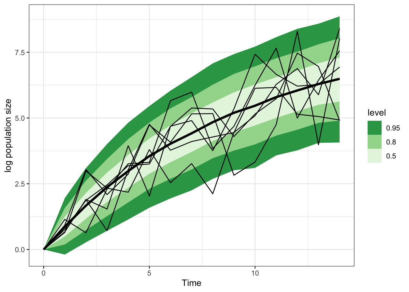

gomp_ar_1_sample$summary(variables = c("a", "b", "sigma",
                                       "mu_max", "sigma_max")) |> 
  knitr::kable()

variable	mean	median	sd	mad	q5	q95	rhat	ess_bulk	ess_tail
a	0.8755229	0.8715515	0.0653034	0.0640476	0.7744877	0.9901877	1.002237	1274.784	1329.060
b	0.8919885	0.8926680	0.0188091	0.0186207	0.8595486	0.9219138	1.002168	1276.568	1300.837
sigma	0.5386121	0.5334915	0.0482727	0.0461511	0.4668362	0.6243722	1.004019	1438.492	1641.133
mu_max	8.2620125	8.1184950	0.9562658	0.8650823	6.9728300	10.0094000	1.002092	1446.378	1782.139
sigma_max	1.2005219	1.1903850	0.1052177	0.1015655	1.0467550	1.3880110	1.002135	1844.450	1556.341

Say it again but different: parameterizing based on \(\mu\) and \(\sigma\)

It might be easier to set priors directly on equilibrium population size (\(\mu_\infty\)) and variance at equilibrium (\(v_\infty\)) so I experimented with parameterizing the model directly that way. It works just as well!

# load the model in stan
ar1_mu_sigma <- cmdstan_model(here::here("posts/2023-11-15-ives03-ts/ar1_mu_sigma.stan"))

ar1_mu_sigma

data{
  int n;
  vector[n] time;
  vector[n] x;
}
// transformed data {
//   vector[n] x = log(pop);
// }
parameters {
  real mu_max;
  real<lower=0,upper=1> b;
  real<lower=0> sigma_max;
}
transformed parameters {
  // real mu_max = a / (1 - b);
  // real sigma_max = sigma /sqrt(1 - b^2);
}
model {
  mu_max ~ normal(7, .5);
  b ~ beta(5,2);
  sigma_max ~ exponential(1);
  x ~ normal(
    mu_max .* (1 - pow(b, time)),
    sigma_max .* sqrt(1 - pow(b^2, time))
    );
}
generated quantities {
  vector[15] x_pred;
  x_pred[1] = 0;
  for (j in 1:14) {
    x_pred[j+1] = normal_rng(
      mu_max * (1 - pow(b, j)),
      sigma_max * sqrt(1 - pow(b^2, j))
      );
  }
}

gomp_ar1_mu_sigma_sample <- ar1_mu_sigma$sample(
  data = list(n = nrow(gomp_nozero),
              x = gomp_nozero$N,
              time = gomp_nozero$time),
  parallel_chains = 4, refresh = 0)

Running MCMC with 4 parallel chains...

Chain 1 finished in 1.3 seconds.
Chain 2 finished in 1.3 seconds.
Chain 3 finished in 1.2 seconds.
Chain 4 finished in 1.2 seconds.

All 4 chains finished successfully.
Mean chain execution time: 1.2 seconds.
Total execution time: 1.5 seconds.

gomp_ar1_mu_sigma_sample |> 
  spread_rvars(x_pred[time]) |> 
  ggplot(aes(x = time-1, ydist = x_pred)) + 
  stat_lineribbon() + 
  scale_fill_brewer(palette = "Greens", direction = -1) + 
  theme_bw() + 
  geom_line(aes(x = time, y = N, group = sim_id),
            inherit.aes = FALSE, data = gomp_one_pop_df)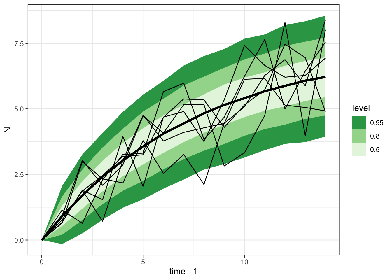

gomp_ar1_mu_sigma_sample$summary(variables = c("mu_max", "b", "sigma_max")) |> 
  knitr::kable()

variable	mean	median	sd	mad	q5	q95	rhat	ess_bulk	ess_tail
mu_max	7.4195465	7.408785	0.3897996	0.3887970	6.8015800	8.0852720	1.003136	1324.390	1827.973
b	0.8758691	0.876516	0.0121230	0.0118971	0.8543245	0.8948875	1.002905	1356.657	1740.710
sigma_max	1.1726875	1.167125	0.0945322	0.0938486	1.0264060	1.3328110	1.000760	2029.433	1859.360

More than one model at once

Here is a no-pooling approach to modelling different clones.

ar1_multispp <- cmdstan_model(here::here("posts/2023-11-15-ives03-ts/ar1_multispp.stan"))
ar1_multispp

data{
  int n;
  int nclone;
  vector[n] time;
  vector[n] x;
  array[n] int<lower=1, upper=nclone> clone_id;
}
// transformed data {
//   vector[n] x = log(pop);
// }
parameters {
  vector[nclone] log_a;
  vector[nclone] logit_b;
  vector[nclone] log_sigma;
}
transformed parameters {
  vector[nclone] b = inv_logit(logit_b);
  vector[nclone] mu_max = exp(log_a) ./ (1 - b);
  vector[nclone] sigma_max = exp(log_sigma) ./ sqrt(1 - b^2);
}
model {
  log_a ~ normal(.7, .2);
  logit_b ~ normal(1, .2);
  log_sigma ~ normal(-1.5, .5);
  x ~ normal(
    mu_max[clone_id] .* (1 - pow(b[clone_id], time)),
    sigma_max[clone_id] .* sqrt(1 - pow(b[clone_id]^2, time))
    );
}
generated quantities {
  matrix[15, nclone] x_pred;
  x_pred[1,] = rep_row_vector(0, nclone);
  for (s in 1:nclone){
    for (j in 1:14) {
      x_pred[j+1,s] = normal_rng(
        mu_max[s] .* (1 - pow(b[s], j)),
        sigma_max[s] .* sqrt(1 - pow(b[s]^2, j))
        );
    }
  }
}

A few things are different in this model compared to the previous one:

• I’m passing in ID numbers for each clone, and an integer number for maximum number of clones
• the model parameters are now vectors, not scalars
• I’ve also put the parameters on different scale. This will come in handy later when the model becomes hierarchical. Whenever I personally do this, I also change the names (see Note below).
• The predictions are now a matrix. This is because we need two different pieces of information for each observation: what time it is, and which clone we’re talking about.

Call me by your name

This code shows off a habit I’ve developed over the last few months of working on Bayesian models. When I put a parameter on a link scale, I change the parameter name to add the name of that link scale.

For example, you might have a strictly positive parameter and model it like this:

parameters {
  real<lower=0> alpha;
}
model {
  alpha ~ normal(1, .5);
  ....
}

But then you might decide to model that on a log scale, either to reparameterize or to prepare for making it hierarchical later. Using link functions like the log and logit is standard in hiearchical models because it allows us to calculate a different value for every group, above and below the overall average, while respecting any constraints

parameters {
  real alpha_log;
}
model {
  alpha_log ~ normal(0, .2);
}

I don’t usually try to make sure the prior is EXACTLY equivalent, but its usually pretty straightforward to get kind of close.

To validate this model, I’m going to generate 6 aphid clones by choosing parameters for a and b from different

as <- runif(n = 6, min = 1.5, max = 2.5)
bs <- runif(n = 6, min = .4, max = .9)
gomp_many_df <- expand_grid(clone_id = 1:6, rep_id = 1:10) |> 
  mutate(a = as[clone_id],
         b = bs[clone_id]) |> 
  rowwise() |> 
  mutate(x = list(sim_one_gompertz(a = a, b = b)))

gomp_nozero_many_df <- gomp_many_df  |> 
  unnest(x) |> 
    filter(time != 0)

gomp_nozero_many_df |> 
  ggplot(aes(x = time, y = N, group = rep_id)) + 
  geom_line() + 
  facet_wrap(~clone_id)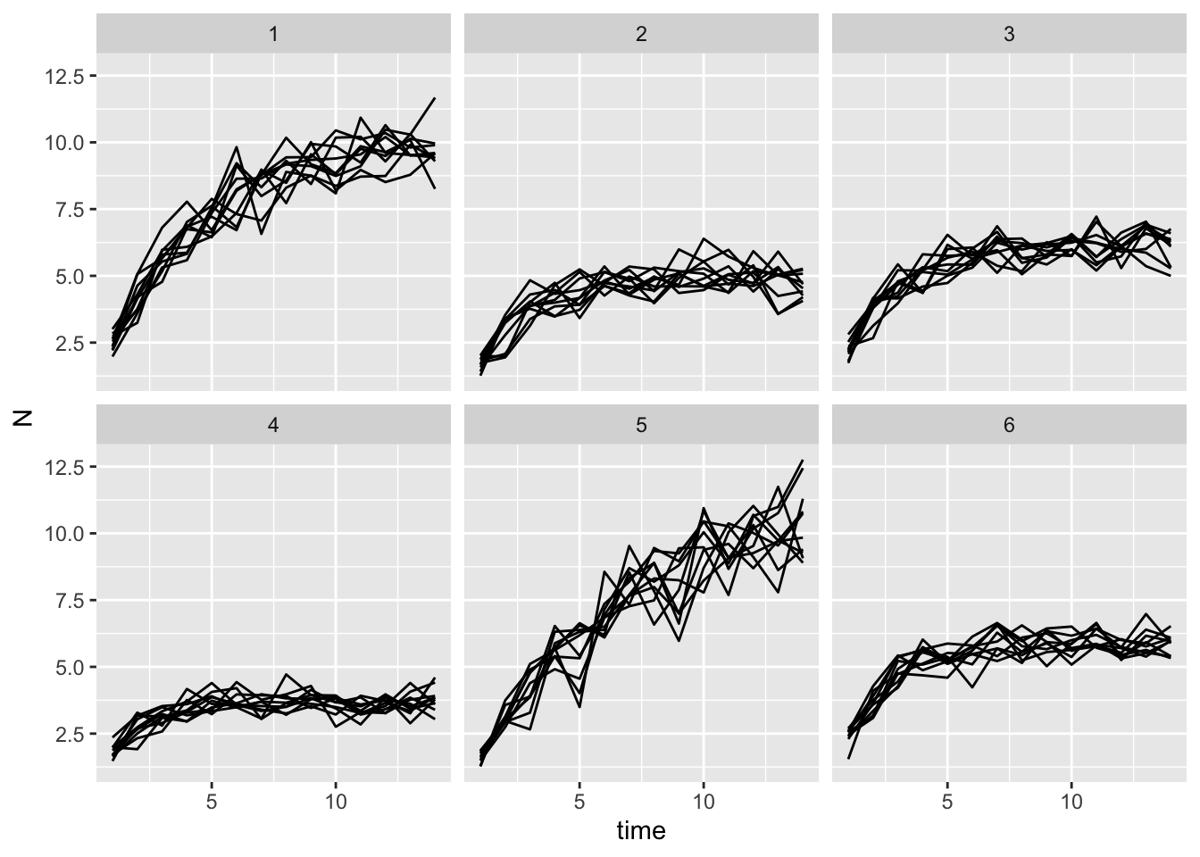

ar1_multispp_samp <- ar1_multispp$sample(
  data = list(n = nrow(gomp_nozero_many_df),
              nclone = max(gomp_nozero_many_df$clone_id),
              time = gomp_nozero_many_df$time,
              x = gomp_nozero_many_df$N,
              clone_id = gomp_nozero_many_df$clone_id), 
  parallel_chains = 4,
  refresh = 0
)

Running MCMC with 4 parallel chains...

Chain 2 finished in 23.8 seconds.
Chain 1 finished in 24.2 seconds.
Chain 3 finished in 24.1 seconds.
Chain 4 finished in 24.1 seconds.

All 4 chains finished successfully.
Mean chain execution time: 24.0 seconds.
Total execution time: 24.3 seconds.

ar1_multispp_samp

   variable  mean median   sd  mad    q5   q95 rhat ess_bulk ess_tail
 lp__       79.64  79.98 3.07 3.01 74.05 84.00 1.00     1728     2506
 log_a[1]    0.86   0.86 0.02 0.02  0.83  0.90 1.00     4228     2969
 log_a[2]    0.58   0.58 0.03 0.03  0.52  0.63 1.00     4768     2881
 log_a[3]    0.79   0.79 0.03 0.03  0.75  0.83 1.00     4648     2895
 log_a[4]    0.56   0.56 0.03 0.03  0.50  0.61 1.00     4467     2727
 log_a[5]    0.52   0.51 0.03 0.03  0.47  0.57 1.00     4103     3076
 log_a[6]    0.85   0.85 0.03 0.02  0.81  0.90 1.00     4921     2812
 logit_b[1]  1.17   1.17 0.04 0.04  1.10  1.24 1.00     4148     2972
 logit_b[2]  0.59   0.59 0.06 0.06  0.48  0.69 1.00     4790     2715
 logit_b[3]  0.59   0.59 0.05 0.05  0.51  0.67 1.00     4720     2849

 # showing 10 of 127 rows (change via 'max_rows' argument or 'cmdstanr_max_rows' option)

ar1_multispp_samp |> 
  gather_rvars(x_pred[time,clone_id]) |> 
  ggplot(aes(x = time-1, ydist = .value)) + stat_lineribbon() + 
  facet_wrap(~clone_id) + 
  scale_fill_brewer(palette = "Greens") + 
  ## add data
  geom_line(aes(x = time, y = N, group = rep_id), 
            data = gomp_nozero_many_df,
            inherit.aes = FALSE)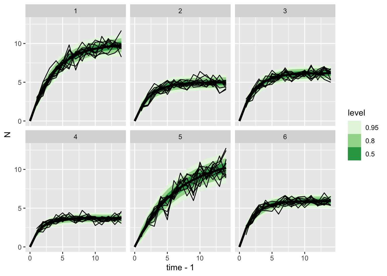 

Time equals 🫖 - 1

One of the trickiest parts of working with these models has been adding and subtracting \(1\). Here’s some notes for the next time I get confused:

• take out the first value We can’t use data including time=0 in a stan model because that implies 0 variance, which just causes lots of errors with the normal likelihood. Taking this point out is no loss, because it doesn’t give us any real information – there’s no variance at all.
• using position in the matrix as data for predictions I generate predictions for new clonal lines, in order to generate the posterior predictive distribution and plot the figures. I store these predictions in a matrix. However, the first observation (time = 0) is actually stored in the first position of the matrix (i.e., row 1). I just evaluate time as all the integers between 0 and 14, which gives two weeks of experiment in this case. You can see in the generated quantities block that I actually use the index value in the for-loop (I called it j) as the value of time. This requires a weird trick: the value of j gets used, but then it is placed in the j+1 position in the vector. This is because there is no “row 0” to go with the observation at time 0, so everything is pushed up by 1.
• subtract 1 to get the correct time This means that to get the right time, we need to subtract 1 from the value used in generated quantities. When I use tidybayes to extract the predictive distribution, I use gather_rvars(x_pred[time,clone_id]) to specify that I want to call the first dimension of the matrix “time”, and the second “clone_id”. But then when I plot these data, I need to subtract 1 from the row position of a prediction to get the actual time value. This is because time = 0 is in row 1, time = 1 is in row 2, etc. Doing this gives a figure where model predictions match

Hierarchical model

ar1_multilevel <- cmdstan_model(here::here("posts/2023-11-15-ives03-ts/ar1_multilevel.stan"))
ar1_multilevel

// modified from previous models with help from ChatGPT!
data {
  int n;
  int nclone;
  vector[n] time;
  vector[n] x;
  array[n] int<lower=1, upper=nclone> clone_id;
}
transformed data{
  vector[n] twotime = 2 * time;
}
parameters {
  vector[nclone] mu_log_a;
  vector[nclone] mu_logit_b;
  vector[nclone] mu_log_sigma;

  cholesky_factor_corr[3] L_corr;  // Cholesky factorization of the correlation matrix
  vector<lower=0>[3] sigma_params;  // Standard deviations for log_a, logit_b, log_sigma

  matrix[nclone, 3] z_params_raw;  // Unconstrained parameters
}

transformed parameters {
  matrix[nclone, 3] z_params = z_params_raw * diag_pre_multiply(sigma_params, L_corr);

  vector[nclone] log_a = mu_log_a + z_params[,1];
  vector[nclone] logit_b = mu_logit_b + z_params[,2];
  vector[nclone] log_sigma = mu_log_sigma + z_params[,3];

  vector[nclone] b = inv_logit(logit_b);
  vector[nclone] mu_max = exp(log_a - log1m_inv_logit(b));
  vector[nclone] sigma_max = exp(log_sigma) ./ sqrt(1 - square(b));
}

model {
  mu_log_a ~ normal(0.7, 0.2);
  mu_logit_b ~ normal(1.7, 0.2);
  mu_log_sigma ~ normal(-.7, 0.25);

  L_corr ~ lkj_corr_cholesky(4);  // Prior on the Cholesky factor for the correlation matrix

  sigma_params[1] ~ exponential(4);
  sigma_params[2] ~ exponential(4);
  sigma_params[3] ~ exponential(3.5);

  to_vector(z_params_raw) ~ std_normal();

  x ~ normal(
    mu_max[clone_id] .* (1 - pow(b[clone_id], time)),
    sigma_max[clone_id] .* sqrt(1 - pow(b[clone_id], twotime))
  );
}

generated quantities {
  matrix[15, nclone] x_pred;
  x_pred[1,] = rep_row_vector(0, nclone);
  for (s in 1:nclone){
    for (j in 1:14) {
      x_pred[j+1,s] = normal_rng(
        mu_max[s] .* (1 - pow(b[s], j)),
        sigma_max[s] .* sqrt(1 - pow(b[s]^2, j))
      );
    }
  }
}

ar1_multilevel_samp <- ar1_multilevel$sample(
  data = list(n = nrow(gomp_nozero_many_df),
              nclone = max(gomp_nozero_many_df$clone_id),
              time = gomp_nozero_many_df$time,
              x = gomp_nozero_many_df$N,
              clone_id = gomp_nozero_many_df$clone_id), 
  parallel_chains = 4,
  refresh = 500
)

ar1_multilevel_samp

We can fit to previous simulations no problem, but we can also simulate data directly from the model. Because this has gotten kind of big, I’m going to make a Stan program just for simulating data

ar1_multilevel_prior <- cmdstan_model(here::here("posts/2023-11-15-ives03-ts/ar1_multilevel_prior.stan"))
ar1_multilevel_prior

// modified from previous models with help from ChatGPT!
data {
  int nclone;
  int nrep;
}

parameters {
  vector[nclone] mu_log_a;
  vector[nclone] mu_logit_b;
  vector[nclone] mu_log_sigma;

  cholesky_factor_corr[3] L_corr;  // Cholesky factorization of the correlation matrix
  vector<lower=0>[3] sigma_params;  // Standard deviations for log_a, logit_b, log_sigma

  matrix[nclone, 3] z_params_raw;  // Unconstrained parameters
}

transformed parameters {
  matrix[nclone, 3] z_params = z_params_raw * diag_pre_multiply(sigma_params, L_corr);

  vector[nclone] log_a = mu_log_a + z_params[,1];
  vector[nclone] logit_b = mu_logit_b + z_params[,2];
  vector[nclone] log_sigma = mu_log_sigma + z_params[,3];

  vector[nclone] b = inv_logit(logit_b);
  vector[nclone] mu_max = exp(log_a - log1m_inv_logit(b));
  vector[nclone] sigma_max = exp(log_sigma) ./ sqrt(1 - square(b));
}

model {
  mu_log_a ~ normal(0.7, 0.2);
  mu_logit_b ~ normal(1.7, 0.2);
  mu_log_sigma ~ normal(-.7, 0.25);

  L_corr ~ lkj_corr_cholesky(4);  // Prior on the Cholesky factor for the correlation matrix

  sigma_params[1] ~ exponential(4);
  sigma_params[2] ~ exponential(4);
  sigma_params[3] ~ exponential(3.5);

  to_vector(z_params_raw) ~ std_normal();
}

generated quantities {
  array[nclone, nrep, 15] real x_pred;
  for (s in 1:nclone){
    for (r in 1:nrep){
      x_pred[s, r, 1] = 0;
    }
  }
  for (s in 1:nclone){
    for (r in 1:nrep){
      for (j in 1:14) {
        x_pred[s, r, j+1] = normal_rng(
          mu_max[s] .* (1 - pow(b[s], j)),
          sigma_max[s] .* sqrt(1 - pow(b[s]^2, j))
          );
      }
    }
  }
}

This model code lacks the likelihood, but uses the same configuration as the previous non-centered model. It also has a bit more going on the Generated Quantities block. Here, we are simulating multiple replicates using each clone, which simulates the actual experiment.

We can sample from this prior distribution and visualize it to see what it says. This is really the only way to get a good idea of what priors really mean in a nonlinear model like this one!

multilevel_prior <- ar1_multilevel_prior$sample(
  data = list(nclone = 12, nrep = 10), 
  chains = 1,
  refresh = 0)

Running MCMC with 1 chain...

Chain 1 finished in 1.5 seconds.

prior_pred_multilevel <- multilevel_prior |> 
  gather_draws(x_pred[clone_id, rep, time], ndraws = 1) |> 
  mutate(time = time -1)

prior_pred_multilevel |> 
  ggplot(aes(x = time, y = .value, group = rep)) + 
  geom_line() + 
  facet_wrap(~clone_id)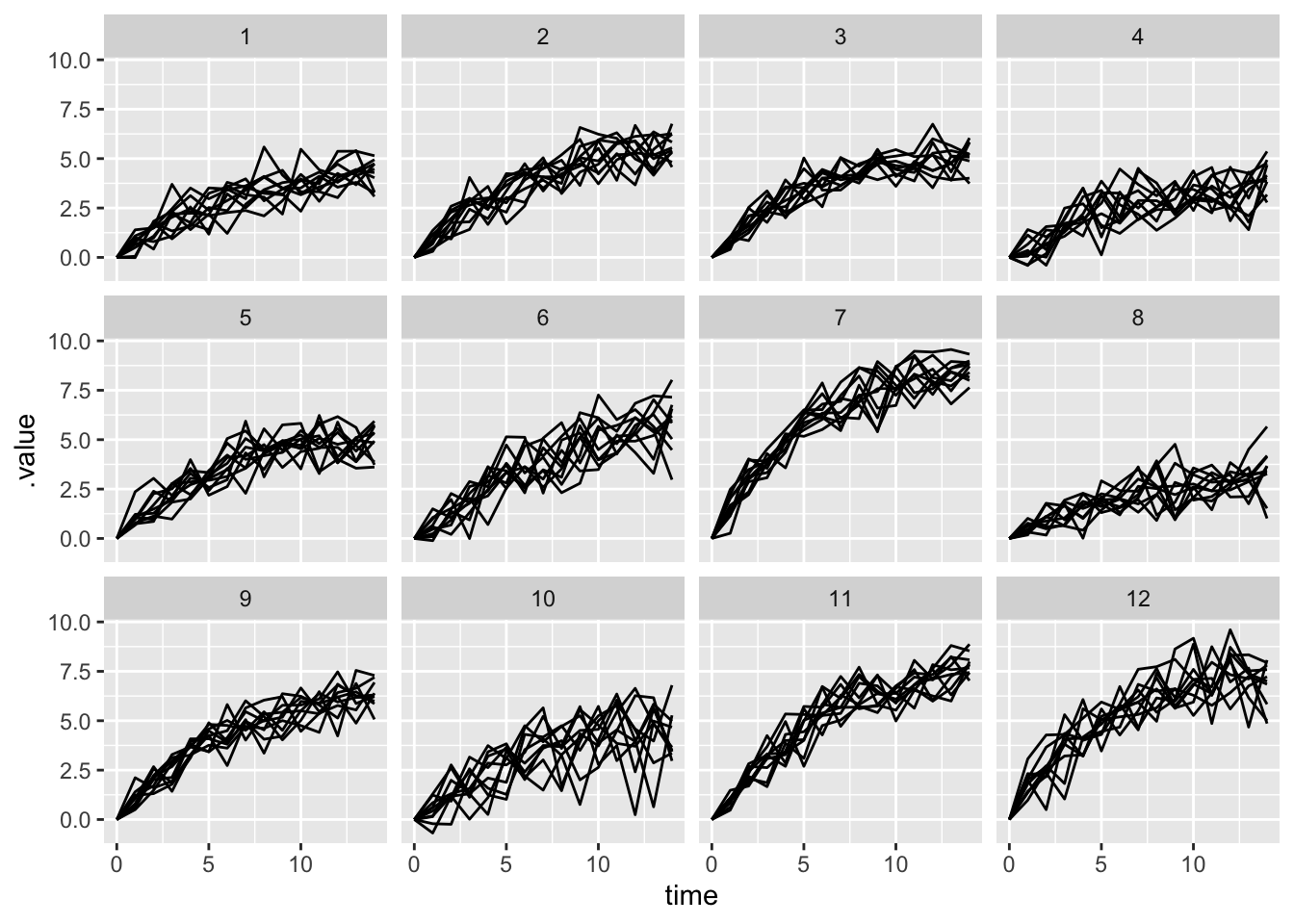

Finally we can put this model through a very similar process of fitting and plotting as previous. Here I’m doing data prep, sampling and plotting all in one plot.

prior_df <- prior_pred_multilevel |> 
  filter(time != 0)

ar1_multilevel_samp <- ar1_multilevel$sample(
  data = list(n = nrow(prior_df),
              nclone = max(prior_df$clone_id),
              time = prior_df$time,
              x = prior_df$.value,
              clone_id = prior_df$clone_id), 
  parallel_chains = 4,
  refresh = 0
)

Running MCMC with 4 parallel chains...

Chain 2 finished in 466.2 seconds.
Chain 3 finished in 472.9 seconds.
Chain 4 finished in 473.9 seconds.
Chain 1 finished in 475.6 seconds.

All 4 chains finished successfully.
Mean chain execution time: 472.2 seconds.
Total execution time: 475.6 seconds.

# ar1_multilevel_samp

ar1_multilevel_samp |> 
  gather_rvars(x_pred[time,clone_id]) |> 
  ggplot(aes(x = time-1, ydist = .value)) + stat_lineribbon() + 
  facet_wrap(~clone_id) + 
  scale_fill_brewer(palette = "Greens") + 
  ## add data
  geom_line(aes(x = time, y = .value, group = rep), 
            data = prior_pred_multilevel,
            inherit.aes = FALSE, col = "darkorange", alpha = .3)  + 
  labs(y = "Population size (log)", 
       x = "Time")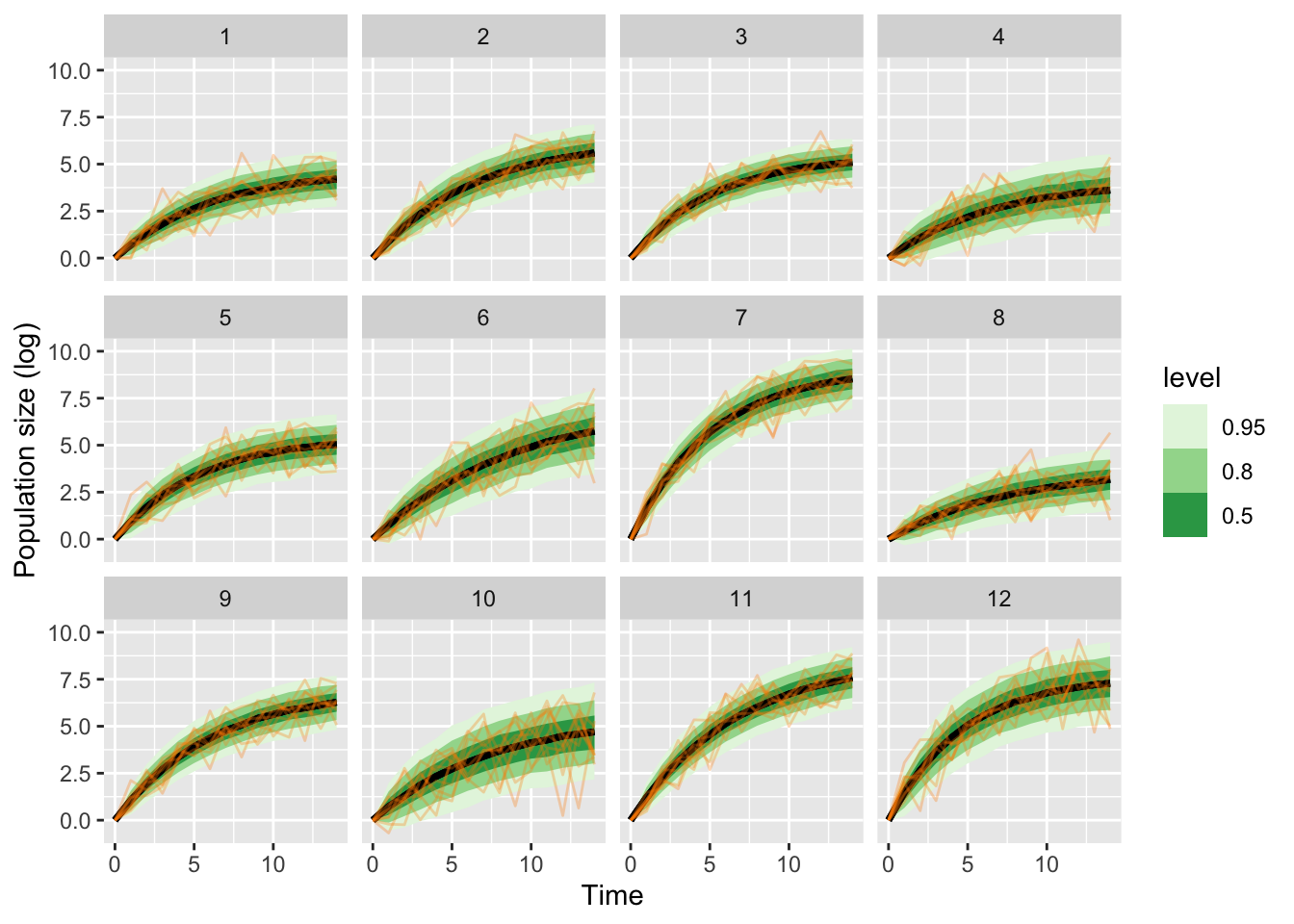

Note that this did not work perfectly, even though we are fitting to the prior predictive distribution. There are divergent iterations!

ar1_multilevel_samp$diagnostic_summary()

$num_divergent
[1] 2 2 6 1

$num_max_treedepth
[1] 0 0 0 0

$ebfmi
[1] 0.8415368 1.0193399 0.8426104 0.9076898

References

Ives, A. R., B. Dennis, K. L. Cottingham, and S. R. Carpenter. 2003. “ESTIMATING COMMUNITY STABILITY AND ECOLOGICAL INTERACTIONS FROM TIME-SERIES DATA.” Ecological Monographs 73 (2): 301–30. https://doi.org/10.1890/0012-9615(2003)073[0301:ECSAEI]2.0.CO;2.