Stan-dalone generated quantites

library(cmdstanr)
library(ggplot2)
library(tidyverse)
library(tidybayes)

Breaking apart Stan programs

Sometimes we don’t want the output of a Stan model to become enormous. However, Stan models can be very convenient for calculating generated quantities. Of course this can be done in R, but sometimes it is just easier to have all the outputs presented in the same way.

See a description of this in the User’s guide and in the CmdStanR help file

example: Marginal effects in multiple regression

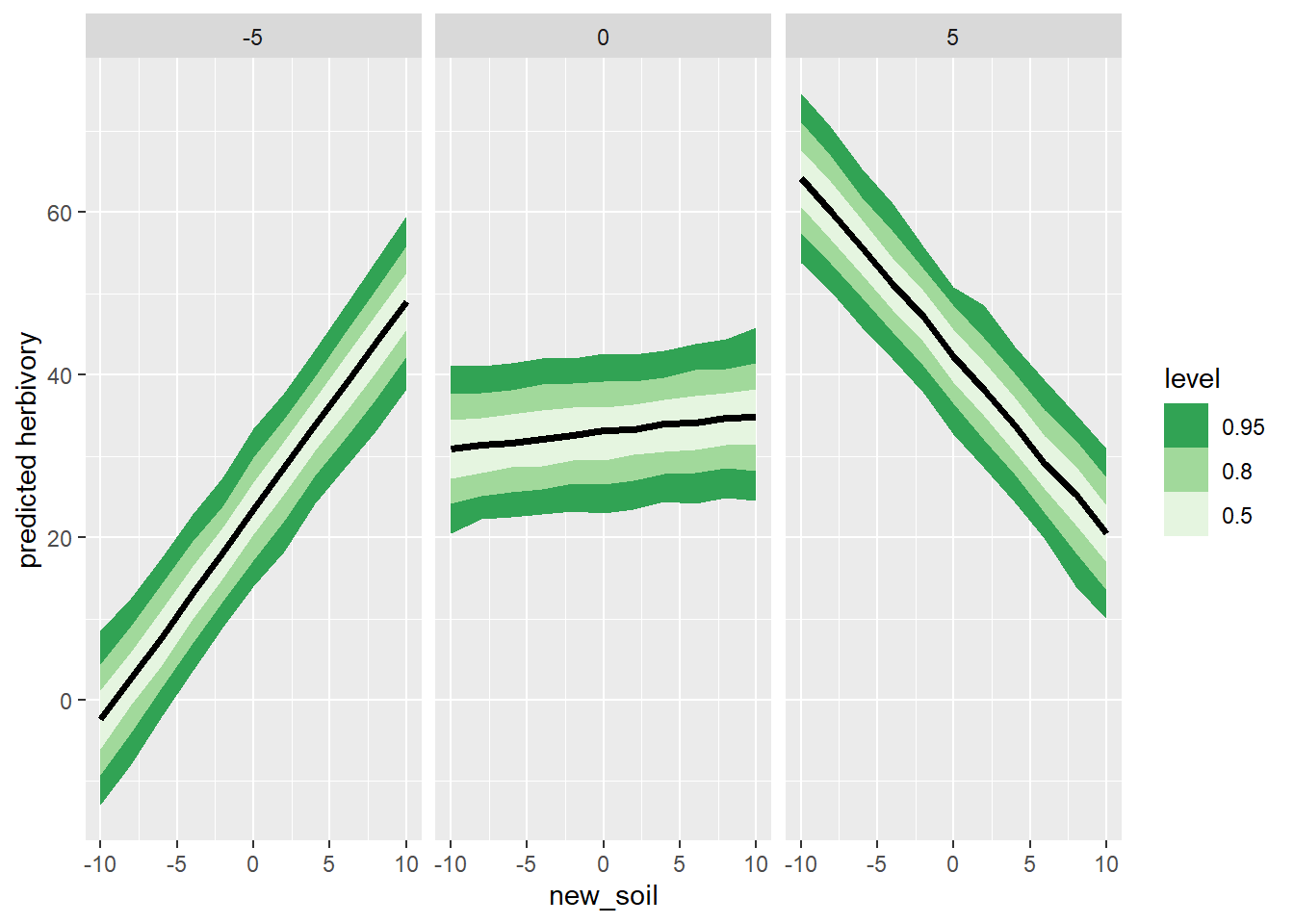
Suppose there is a plant which, when growing in N-rich soil, is able to generate chemical defenses to prevent damage by a herbivorous insect. On poor soil the herbivore eats much more of the plant

set.seed(4812)
soil_quality <- runif(200, min = -3, max = 3)
insect_biomass <- runif(200, min = -10, max = 10)
# each gram of insect biomass eats 1.2 grams of plant biomass
insect_eff_per_g <- 2

soil_quality_eff_per_unit <- 0

soil_quality_on_herb <- -.5

herb_avg_soil_avg_density <- 33

mu_herbivory <- herb_avg_soil_avg_density + 
  soil_quality_eff_per_unit* soil_quality + 
  (insect_eff_per_g + soil_quality_on_herb*soil_quality) * insect_biomass 

sigma_herb <- 5
obs_herbivory <- rnorm(n = 200, mu_herbivory, sigma_herb)

tibble(soil_quality, insect_biomass, obs_herbivory) |> 
  ggplot(aes(x = soil_quality, y = obs_herbivory, col = insect_biomass)) + 
  geom_point()

Here is a Stan program to model this interaction

# class-output: stan

multiple_regression <- cmdstan_model(
  here::here(
    "posts/2023-11-01-standalone-gq/multiple_regression.stan"
    ))

multiple_regression

data{
  int<lower=0> n;
  vector[n] soil;
  vector[n] insects;
  vector[n] herbivory;
}
parameters{
  real avg_herb;
  vector[3] beta;
  real<lower=0> sigma;
}
model{
  sigma ~ exponential(.25);
  beta ~ std_normal();
  avg_herb ~ normal(30, 5);
  herbivory ~ normal(avg_herb + beta[1]* soil + beta[2]*insects + beta[3]*(soil .* insects), sigma);
}

multiple_post <- multiple_regression$sample(data = list(n = length(soil_quality), soil = soil_quality, insects = insect_biomass, herbivory = obs_herbivory), parallel_chains = 2, refresh = 0)

Running MCMC with 4 chains, at most 2 in parallel...

Chain 1 finished in 0.3 seconds.
Chain 2 finished in 0.2 seconds.
Chain 3 finished in 0.2 seconds.
Chain 4 finished in 0.2 seconds.

All 4 chains finished successfully.
Mean chain execution time: 0.2 seconds.
Total execution time: 0.8 seconds.

We can see that the posteriors are close to the true values (not the point of this post, but always good to check)

multiple_post$summary()

# A tibble: 6 × 10
  variable     mean   median     sd    mad       q5      q95  rhat ess_bulk
  <chr>       <num>    <num>  <num>  <num>    <num>    <num> <num>    <num>
1 lp__     -416.    -415.    1.63   1.48   -419.    -414.     1.00    1904.
2 avg_herb   32.9     32.9   0.336  0.333    32.4     33.5    1.00    3855.
3 beta[1]     0.192    0.190 0.191  0.192    -0.123    0.507  1.00    4847.
4 beta[2]     1.93     1.93  0.0607 0.0589    1.83     2.03   1.00    4096.
5 beta[3]    -0.474   -0.474 0.0341 0.0345   -0.530   -0.418  1.00    4922.
6 sigma       4.80     4.79  0.238  0.235     4.43     5.20   1.00    4098.
# ℹ 1 more variable: ess_tail <num>

Now suppose we want to plot this interaction. We could do so in R, no problem. We could also do that in the model above. But you might not want to! reasons include:

• keeping the output of any one model small(ish) so that you can actually work with it

# class-output: stan

multi_reg_triptych <- cmdstan_model(
  here::here(
    "posts/2023-11-01-standalone-gq/multi_reg_triptych.stan"
    ))

multi_reg_triptych

data {
  int<lower=0> npred;
  vector[npred] new_soil;
  vector[npred] new_insect;
}
// copied from the previous model!
parameters{
  real avg_herb;
  vector[3] beta;
  real<lower=0> sigma;
}
generated quantities {
  vector[npred] pred_herbivory;
  for (i in 1:npred){
    pred_herbivory[i] = normal_rng(avg_herb + beta[1]* new_soil[i] + beta[2]*new_insect[i] + beta[3]*(new_soil[i] * new_insect[i]), sigma);
  }
}

get the prediction data ready

newdata <- expand_grid(new_insect = c(-5, 0, 5),
            new_soil = seq(from = -10, to = 10, length.out = 11))


multi_trip <- multi_reg_triptych$generate_quantities(
  fitted_params = multiple_post,
  data = list(
    new_insect = newdata$new_insect,
    new_soil = newdata$new_soil,
    npred = nrow(newdata)
  )
)

Running standalone generated quantities after 4 MCMC chains, 1 chain at a time ...

Chain 1 finished in 0.0 seconds.
Chain 2 finished in 0.0 seconds.
Chain 3 finished in 0.0 seconds.
Chain 4 finished in 0.0 seconds.

All 4 chains finished successfully.
Mean chain execution time: 0.0 seconds.
Total execution time: 1.0 seconds.

multi_trip |> 
  gather_rvars(pred_herbivory[i]) |> 
  bind_cols(newdata) |> 
  ggplot(aes(x = new_soil, dist = .value)) + 
  stat_lineribbon() + 
  facet_wrap(~new_insect) + 
  scale_fill_brewer(palette = "Greens", direction = -1) + 
  labs(x = "new_soil", y = "predicted herbivory")

Visualizing an interaction. The effect of soil quality on herbivory varies with herbivore biomass (in a very pretend, make-believe example).