Uncertainty in growth increments

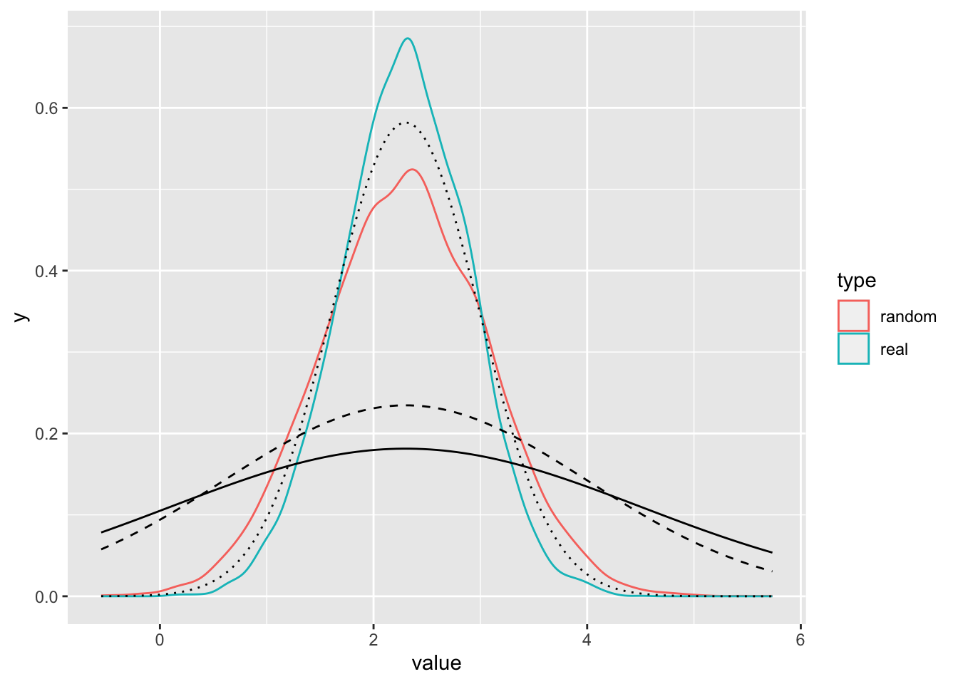
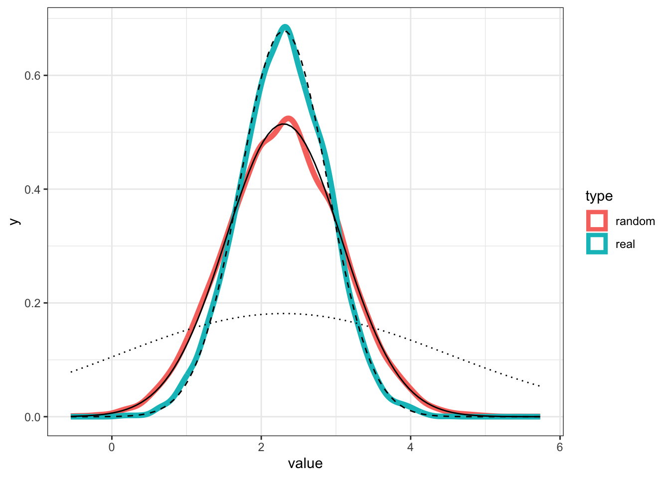
The following is a simulation by Will Vieira which explores how process uncertainty and measurement error combine when we measure trees.

The model imagines a simple linear growth scenario: every year, individuals grow by a random amount \(g_i\). This growth increment is random and varies each year according to a normal distribution

\[ \begin{align} L_{\text{year}[i]} \sim N \\ \end{align} \]

\[ L = lo \]

Here is Will’s very clean and concise simulation code.

library(ggplot2)
library(tidyverse)

set.seed(0.0)

nbInd <- 2000
deltaYear = 14
obsError = 5

# Generate individual trees with random size in mm
sizeGrowth_dt <- tibble(
    tree_id = 1:nbInd,
    size_real0 = rgamma(nbInd, 190^2/1e4, 190/1e4)
    ) |>
    # each indv increment every year with a N(2.3, 2.2) (values from dataset);
    # here from size_t to size_t+1 is the sum of X years growth
    mutate(
        size_real1 = size_real0 + replicate(n(), sum(rnorm(deltaYear, 2.3, 2.2))),
        size_real2 = size_real1 + replicate(n(), sum(rnorm(deltaYear, 2.3, 2.2))),
        size_real3 = size_real2 + replicate(n(), sum(rnorm(deltaYear, 2.3, 2.2))),
        size_real4 = size_real3 + replicate(n(), sum(rnorm(deltaYear, 2.3, 2.2)))
    ) |>
    pivot_longer(
        cols = contains('size'),
        names_to = 'timeStep',
        values_to = 'size_real'
    ) |>
    # each observation has an error of measurement
    mutate(
        size_random = rnorm(n(), mean = size_real, sd = obsError)
    ) |>
    # calculate growth from real and random (observed) values
    group_by(tree_id) |>
    mutate(
        growth_real = (size_real - lag(size_real, 1))/deltaYear,
        growth_random = (size_random - lag(size_random, 1))/deltaYear
    ) |>
    ungroup() |>
    pivot_longer(
        cols = contains(c('real', 'random')),
        names_to = c('var', 'type'),
        names_sep = '_'
    ) |>
    # remove NA for first time step
    filter(!is.na(value))

p1 <- sizeGrowth_dt |>
  pivot_wider(
    names_from = type,
    values_from = value
  ) |>
  ggplot(aes(x = real, y = random)) +
  geom_point(size = .5) +
  facet_wrap(~var, scales = 'free') +
  geom_abline(intercept = 0, slope = 1)

p2 <- sizeGrowth_dt |>
  ggplot(aes(value, color = type)) +
  geom_density() +
  facet_wrap(~var, scales = 'free')

library(patchwork)
p1  + p2

sizeGrowth_dt |> 
  filter(var == "growth") |> 
  ggplot(aes(x = value, colour = type)) + 
  geom_density() + 
  stat_function(fun = function(x) dnorm(x, mean = 2.3, sd = 2.2),
                colour = "black") + 
  stat_function(fun = function(x) dnorm(x, mean = 2.3, sd = sqrt(deltaYear)/2.2),
                colour = "black", lty = 2) + 
  stat_function(fun = function(x) dnorm(x, mean = 2.3, 
                                        sd = sqrt(deltaYear)/sqrt(2.2^2 + obsError^2)),
                colour = "black", lty = 3)

sd_g <- 2.2

sizeGrowth_dt |> 
  filter(var == "growth") |> 
  ggplot(aes(x = value, colour = type)) + 
  geom_density(lwd = 2) + 
  stat_function(fun = function(x) dnorm(x, mean = 2.3, sd = 2.2),
                colour = "black", lty = 3) + 
  stat_function(fun = function(x) dnorm(x, mean = 2.3, sd = 2.2/sqrt(deltaYear)),
                colour = "black", lty = 2) + 
  stat_function(fun = function(x) dnorm(x, mean = 2.3, 
                                        sd = sqrt(
                                          (sd_g^2 * deltaYear + 2*obsError^2)/deltaYear^2
                                          )
                                        ),
                colour = "black", lty = 1) + 
  theme_bw()

but why are these correlated?

Distribution of a difference

u1 <- 8
u2 <- 15
sdx <- 1.5
n <- 1e5
x1 <- rnorm(n, mean = u1, sd = sdx)
x2 <- rnorm(n, mean = u2, sd = sdx)
tibble(diff = x2 - x1) |> 
  ggplot(aes(x = diff)) + 
  stat_function(fun = \(x) dnorm(x, mean = u2 - u1, sd = sqrt(2) * sdx),
                size = 3, col = "darkgreen") + 
  geom_density(size = 1, col = "orange")

Warning: Using `size` aesthetic for lines was deprecated in ggplot2 3.4.0.
ℹ Please use `linewidth` instead.

This is what happens when you have two constant values which are measured with error and then contrasted.

if another process adds to the variation, then the two variances add – THEN get scaled but sqrt(2)