The Cholesky decomposition

library(targets)
library(ggplot2)
library(tidyverse)
library(tidybayes)

You can give uncorrelated random numbers a specific correlation by using the Cholesky decomposition. This comes in handy when you’re modelling correlated random variables using MCMC.

eg <- rethinking::rlkjcorr(1, 2, 1)
eg

          [,1]      [,2]
[1,]  1.000000 -0.351295
[2,] -0.351295  1.000000

cc <- chol(eg)

purrr::rerun(30,{
  zz <- matrix(data = rnorm(500), ncol = 2)
  # plot(zz)
  rr <- t(cc) %*% t(zz)
  # plot(t(rr))
  cor(t(rr))[1,2]
}) |> 
  purrr::flatten_dbl() |> density() |> plot(main = "Simulated correlations")

Warning: `rerun()` was deprecated in purrr 1.0.0.
ℹ Please use `map()` instead.
  # Previously
rerun(30, {
zz <- matrix(data = rnorm(500), ncol = 2)
rr <- t(cc) %*% t(zz)
cor(t(rr))[1, 2]
})

  # Now
map(1:30, ~ {
zz <- matrix(data = rnorm(500), ncol = 2)
rr <- t(cc) %*% t(zz)
cor(t(rr))[1, 2]
})

abline(v=eg[1,2])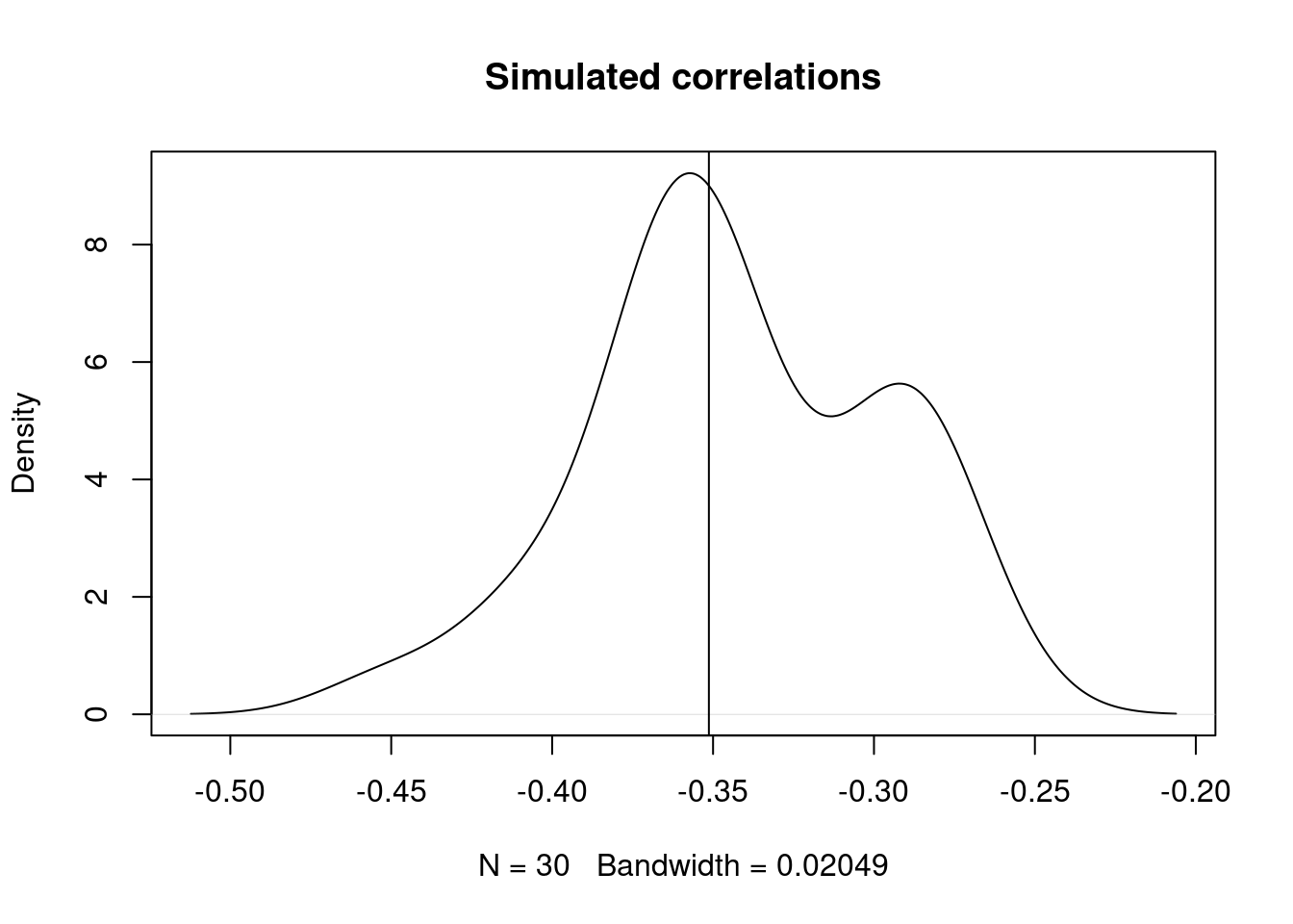

Here we can see that the correlation we want is -0.351295, and indeed we’re able to give exactly that correlation to uncorrelated random numbers.

eg <- rethinking::rlkjcorr(1, 2, 5)
print(eg)
cc <- chol(eg)

t(cc) %*% cc
mm <- matrix(rnorm(4000, mean = 0, sd = 1), ncol = 2)

plot(mm)
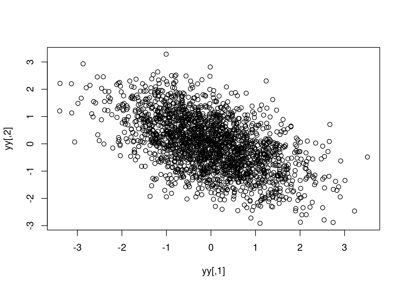
yy <- t(t(cc) %*% t(mm))

plot(yy)

           [,1]       [,2]
[1,]  1.0000000 -0.5282398
[2,] -0.5282398  1.0000000

           [,1]       [,2]
[1,]  1.0000000 -0.5282398
[2,] -0.5282398  1.0000000

uncorrelated numbers

after being given a correlation

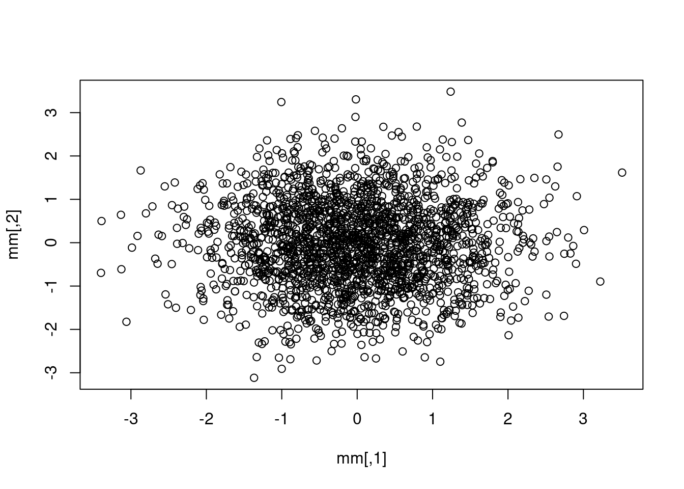
Doing it by hand

Because the case for only two random variables is pretty simple, we can actually write out the Cholesky decomposition by hand. Here I want to give some independent random numbers a correlation of -0.8:

p <- -.8
L <- matrix(c(1,0, p, sqrt(1 - p^2)), ncol = 2, byrow = TRUE)
zz <- matrix(data = rnorm(1000), ncol = 2)
yy <- t(L %*% t(zz))
plot(yy)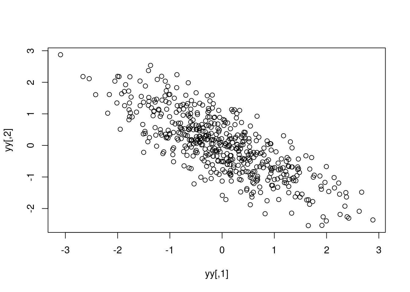

cor(yy)

           [,1]       [,2]
[1,]  1.0000000 -0.7809624
[2,] -0.7809624  1.0000000

This can be written without matrix multiplication like this:

z1 <- rnorm(1000)
z2 <- rnorm(1000)

y1 <- z1
y2 <- p*z1 + sqrt(1 - p^2)*z2

plot(y1, y2)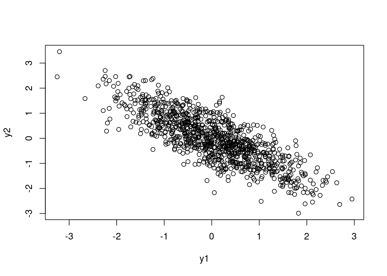

cor(y2, y1)

[1] -0.8054704

In a Stan model, I might want to use a scaled beta distribution to model the correlation between, say, slopes and intercepts in a model:

mu <- .84
phi <- 80
g <- rbeta(1, mu*phi, (1 - mu)*phi)
p_trans <- g*2 - 1

sim_y_corr <- function(n, p) {
  z1 <- rnorm(n)
  z2 <- rnorm(n)
  
  y1 <- z1
  y2 <- p*z1 + sqrt(1 - p^2)*z2
  
  return(data.frame(y1, y2))
}

sim_y_corr(n = 1000, p = p_trans) |> plot()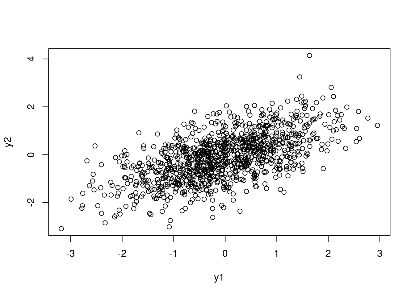

or even work on the logit scale:

q <- rnorm(1, mean = -1, sd = .1)
p_trans_n <- plogis(q)*2 - 1
sim_y_corr(n = 1000, p = p_trans_n) |> plot()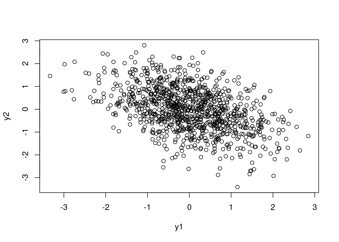

This is even a little easier to think about: because of all the transformations, 0 on the logit scale still means a 0 correlation; negative and positive numbers mean negative and positive correlations as well.

Another way to make correlation matrices is here: https://www.rdatagen.net/post/2023-02-14-flexible-correlation-generation-an-update-to-gencorgen-in-simstudy/