Simple nonlinear growth

library(targets)
library(ggplot2)
library(tidyverse)
library(tidybayes)
suppressPackageStartupMessages(library(brms))

Growth when you know the age

We’re doing a lot of work with growth equations these days! This is how to use brms to fit the growth of an animal when we know:

• the birth year

• size at each year (measured as the length of a leg)

• time

We’ll start with the classic VB growth equation that has been in several other posts:

\[ L_t = L_0e^{-rt} + L_\infty(1 - e^{-rt}) \tag{1}\]

The model we use will resemble the others as well:

\[ \begin{align} \text{Measurements} &\sim \text{Normal}(L_t, \sigma_{meas})\\ L_t &= L_0e^{-rt} + L_\infty(1 - e^{-rt}) \\ L_0 &\sim ...\\ L_\infty &\sim ...\\ r &\sim ... \end{align} \]

Simulating data

I’m starting off with a function to simulate data; this will make it easy to repeat experiments with this model.

simulate_one_growth_known_age <- function(age, r,
                                          Lmax,
                                          size_at_first,
                                          sd_obs){
  tibble(age = 0:age,
         size = size_at_first * exp(-r * age) + Lmax * (1 - exp(-r * age)),
         obs_size = rnorm(n = length(age), mean = size, sd = sd_obs))
}

one_animal <- simulate_one_growth_known_age(9, Lmax = 550, size_at_first = 277, r = .7, sd_obs = 6)

one_animal |> 
  ggplot(aes(x = age, y = obs_size)) + 
  geom_point() + 
  theme_bw() + 
  geom_line(aes(y = size)) + 
  labs(x = "Age", y = "Size")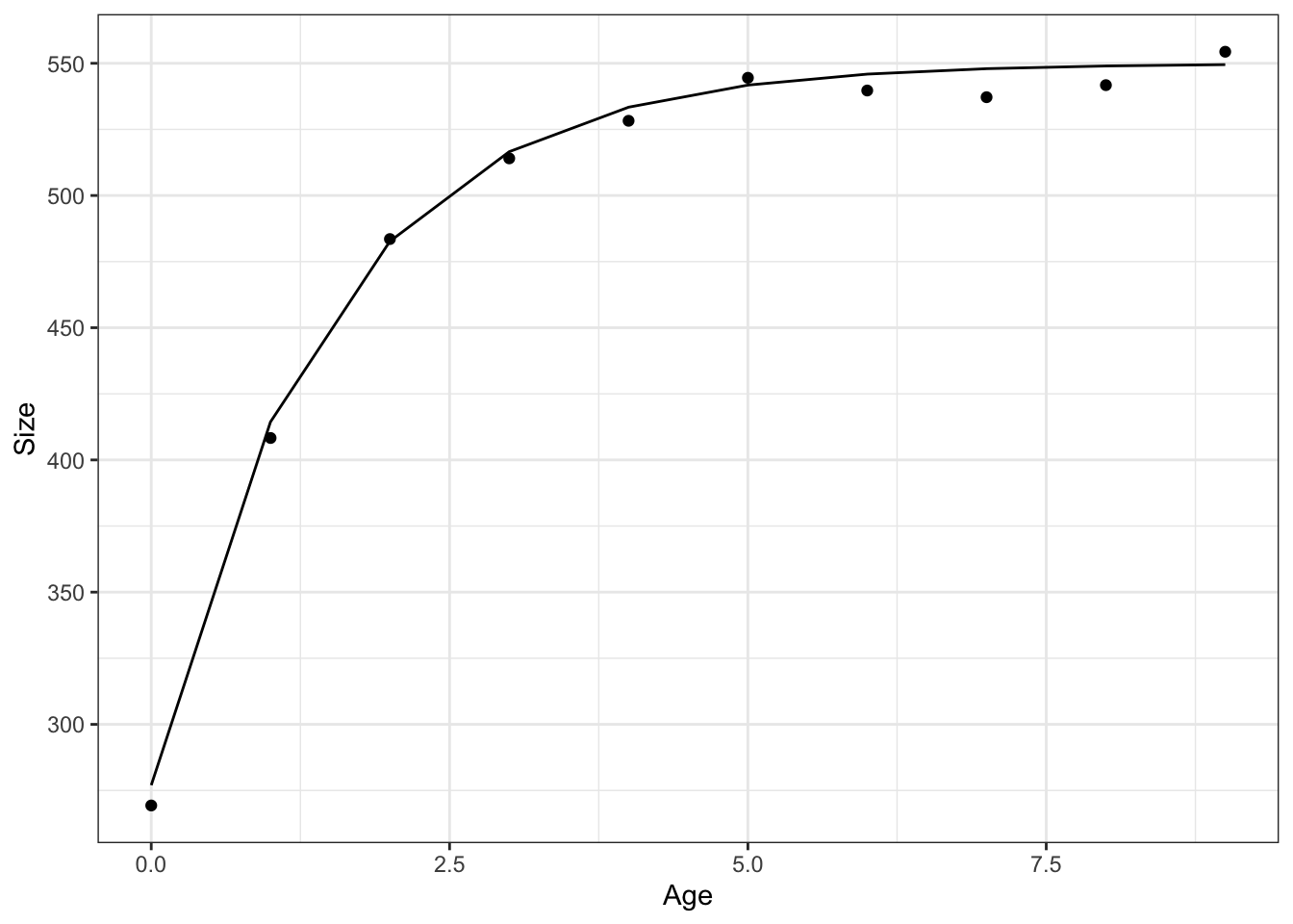 

Growth curve for a single individual. The curved line is the true size, and the dots are observations around it. The observations are taken in the field while the semi-tranquilized animal is struggling, so they show some slight variation.

Nonlinear modelling with BRMS

There are three steps to defining and elementary model with brms:

1. write the model
2. write down some priors
3. condition the model on data

In practice there are many more steps, including prior predictive checks to make sure our priors make sense. In this post I’m going to focus on the mechanistic how-to of fitting a nonlinear model in brms and I’ll come back to Prior Predictive checks, which I love, in another post.

First we define the model, here we need to indicate what are parameters by doing a ~1 after each. Yes it is a formula with multiple little formulae inside it! Feel the power flow through you.

vb_form <- bf(obs_size ~ startsize * exp(-growthrate * age) + maxsize * (1 - exp(-growthrate * age)),
              startsize ~ 1, 
              growthrate ~ 1,
              maxsize ~ 1,
              nl = TRUE,
              family = gaussian())

get_prior(vb_form, data = one_animal)

                 prior class      coef group resp dpar      nlpar lb ub
 student_t(3, 0, 22.6) sigma                                       0   
                (flat)     b                           growthrate      
                (flat)     b Intercept                 growthrate      
                (flat)     b                              maxsize      
                (flat)     b Intercept                    maxsize      
                (flat)     b                            startsize      
                (flat)     b Intercept                  startsize      
       source
      default
      default
 (vectorized)
      default
 (vectorized)
      default
 (vectorized)

vb_prior <- c(
  prior(exponential(1), class = "sigma"),
  prior(normal(0,1), nlpar = "growthrate", lb = 0),
  prior(normal(550, 20), nlpar = "maxsize", lb = 0),
  prior(normal(200, 50), nlpar = "startsize", lb = 0)
)

vb_model <- brm(formula = vb_form,
                prior = vb_prior, 
                data = one_animal, 
                chains = 2, 
                file = here::here("posts/2022-11-21-growth-curve-known-age/vb_model.rds"))

one_animal |> 
  tidybayes::add_predicted_rvars(vb_model) |> 
  ggplot(aes(x = age, dist = .prediction)) + 
  stat_dist_lineribbon() + 
  geom_point(aes(x = age, y = obs_size), inherit.aes = FALSE) 

Warning: Using the `size` aesthietic with geom_ribbon was deprecated in ggplot2 3.4.0.
ℹ Please use the `linewidth` aesthetic instead.

Warning: Unknown or uninitialised column: `linewidth`.

Warning: Using the `size` aesthietic with geom_line was deprecated in ggplot2 3.4.0.
ℹ Please use the `linewidth` aesthetic instead.

Warning: Unknown or uninitialised column: `linewidth`.
Unknown or uninitialised column: `linewidth`.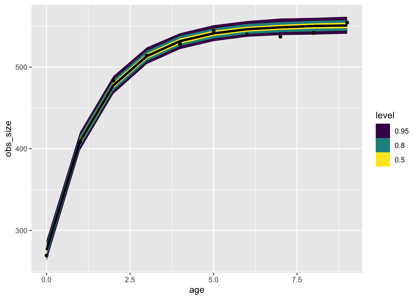

summary(vb_model)

 Family: gaussian 
  Links: mu = identity; sigma = identity 
Formula: obs_size ~ startsize * exp(-growthrate * age) + maxsize * (1 - exp(-growthrate * age)) 
         startsize ~ 1
         growthrate ~ 1
         maxsize ~ 1
   Data: one_animal (Number of observations: 10) 
  Draws: 2 chains, each with iter = 2000; warmup = 1000; thin = 1;
         total post-warmup draws = 2000

Population-Level Effects: 
                     Estimate Est.Error l-95% CI u-95% CI Rhat Bulk_ESS
startsize_Intercept    275.83      4.47   266.81   284.49 1.00     1050
growthrate_Intercept     0.66      0.03     0.61     0.72 1.00      918
maxsize_Intercept      551.62      2.43   546.94   556.62 1.00      814
                     Tail_ESS
startsize_Intercept       866
growthrate_Intercept      796
maxsize_Intercept         765

Family Specific Parameters: 
      Estimate Est.Error l-95% CI u-95% CI Rhat Bulk_ESS Tail_ESS
sigma     4.51      0.96     3.05     6.76 1.00      899      951

Draws were sampled using sampling(NUTS). For each parameter, Bulk_ESS
and Tail_ESS are effective sample size measures, and Rhat is the potential
scale reduction factor on split chains (at convergence, Rhat = 1).